GCG
Branch-and-Price & Column Generation for Everyone
Branch-and-Price & Column Generation for Everyone
If you want to generate visualizations for your experiments (see How to conduct experiments with GCG), you should use the automated generation features of our Visualization Suite. However, you might need to generate single visualizations manually, which is what is explained on this page.
Many different things can be plotted using our visualization framework. You can find all possible arguments here.
In this section, we describe what is required to generate the visualizations using the included visualization scripts. They are also required to be fulfilled if you are only using the Visualization Suite.
The scripts will mostly give helpful error messages if you have misconfigured anything, so please pay attention to their output.
Except for the comparison_table script, all visualizations are generated using python. For those, you need python3 to be installed correctly on your system:
sudo apt-get install python3
For each script, you will need packages and some are probably not yet installed on your computer. You can do that by first installing pip:
sudo apt-get install python3-pip
And then the needed packages via
pip3 install numpy matplotlib pandas sklearn
Furthermore, we recommend to install the package
tqdm
which shows progress bars which can be useful in particular for very large runtime data.
For the pricing visualizations, a working LaTeX installation is required, i.e.
sudo apt-get install dvipng texlive-latex-extra texlive-fonts-recommended
should be up to date.
First, you have to do a testrun to gather the data for the visualizations. A guide on how to do that can be found here.
The scripts sometimes expect a certain flag to be set. The following table gives an overview over the requirements for the runtime data for each visualization script.
| Expected Input | Required compile flags | Required test flags | |
|---|---|---|---|
| Performance Profile | .out/.res | - | - |
| General | .out | - | STATISTICS=true |
| Bounds | .out | STATISTICS=true | STATISTICS=true |
| Classifier/ Detection | .out | - | DETECTIONSTATISTICS=true |
| Pricing | .out, .vbc | STATISTICS=true | - |
| Tree | .vbc | - | |
| Comparison Table | .res | - | - |
You can create different plots with the included scripts in the
statsfolder. All scripts are briefly explained in the following. When describing how to execute them, it is always assumed that you are inside thestatsfolder.
The following arguments are common across all following scripts (except for the performance profile plotter and comparison table).
-o OUTDIR, --outdir OUTDIR
                      output directory (default: "plots")
-save, --savepickle      parses the given .out-file without plotting
-load, --loadpickle      loads the given .pkl-file and plots it
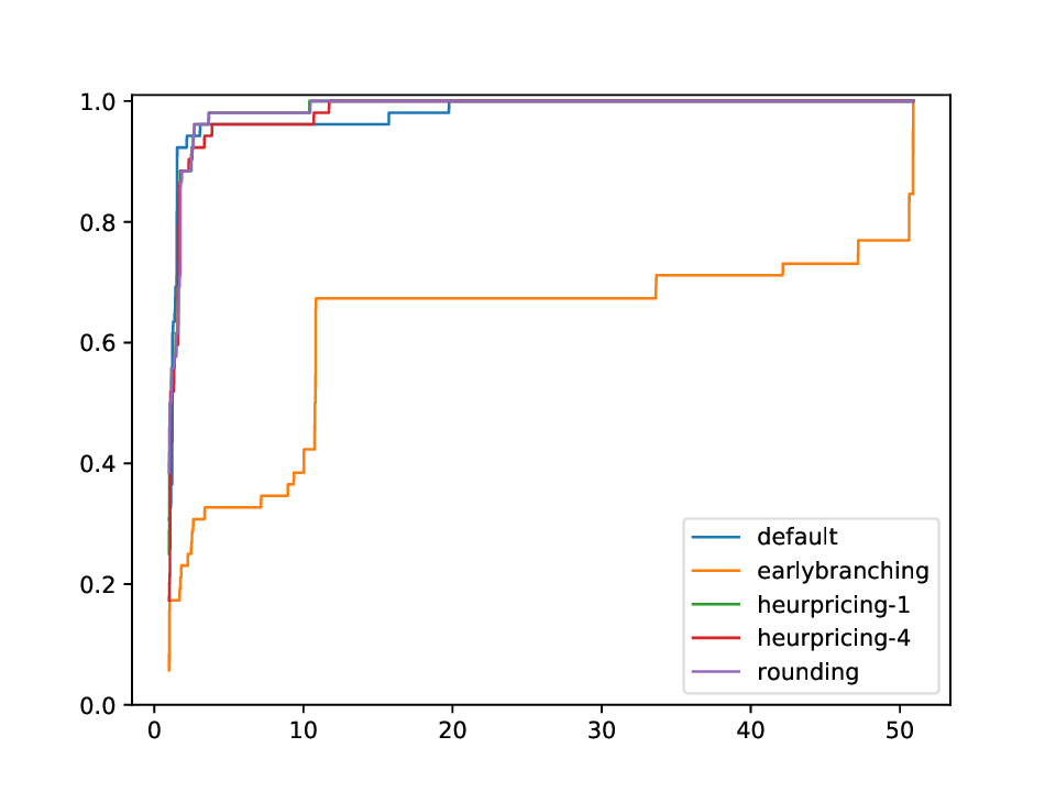
Using this plotter, one can generate performance profiles. In those, the x-axis represents the factor by which the respective run is worse than the optimal run, while the y-axis is the corresponding probability.
python3 general/performance_profile.py FILES
with FILES being some (space-separated) .res or .out files in the format as shown in 'What files do I get'.
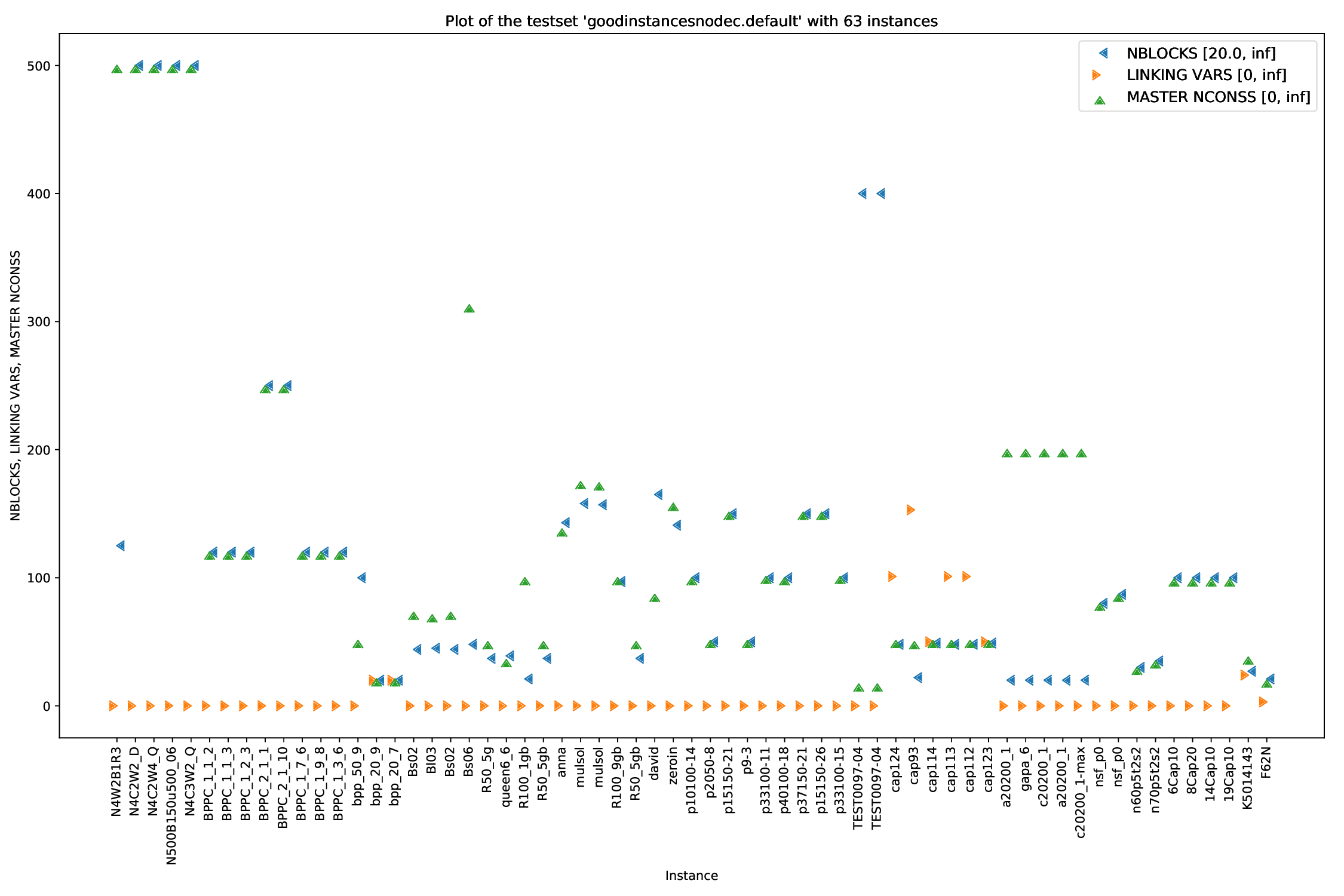
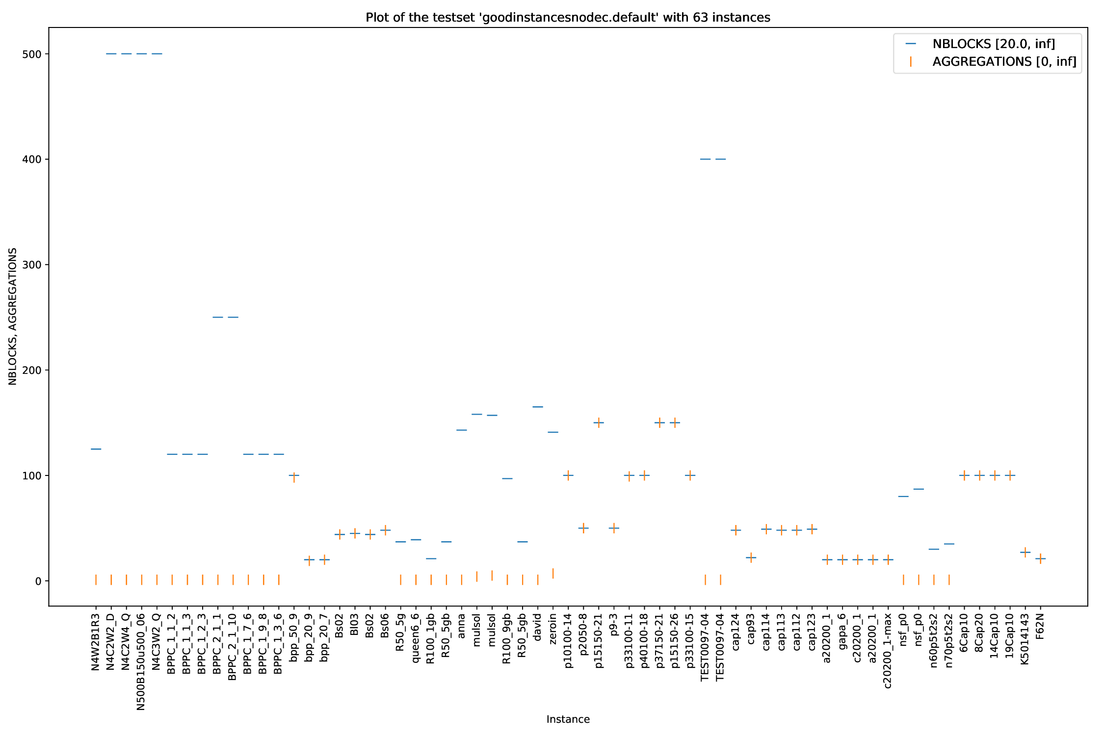
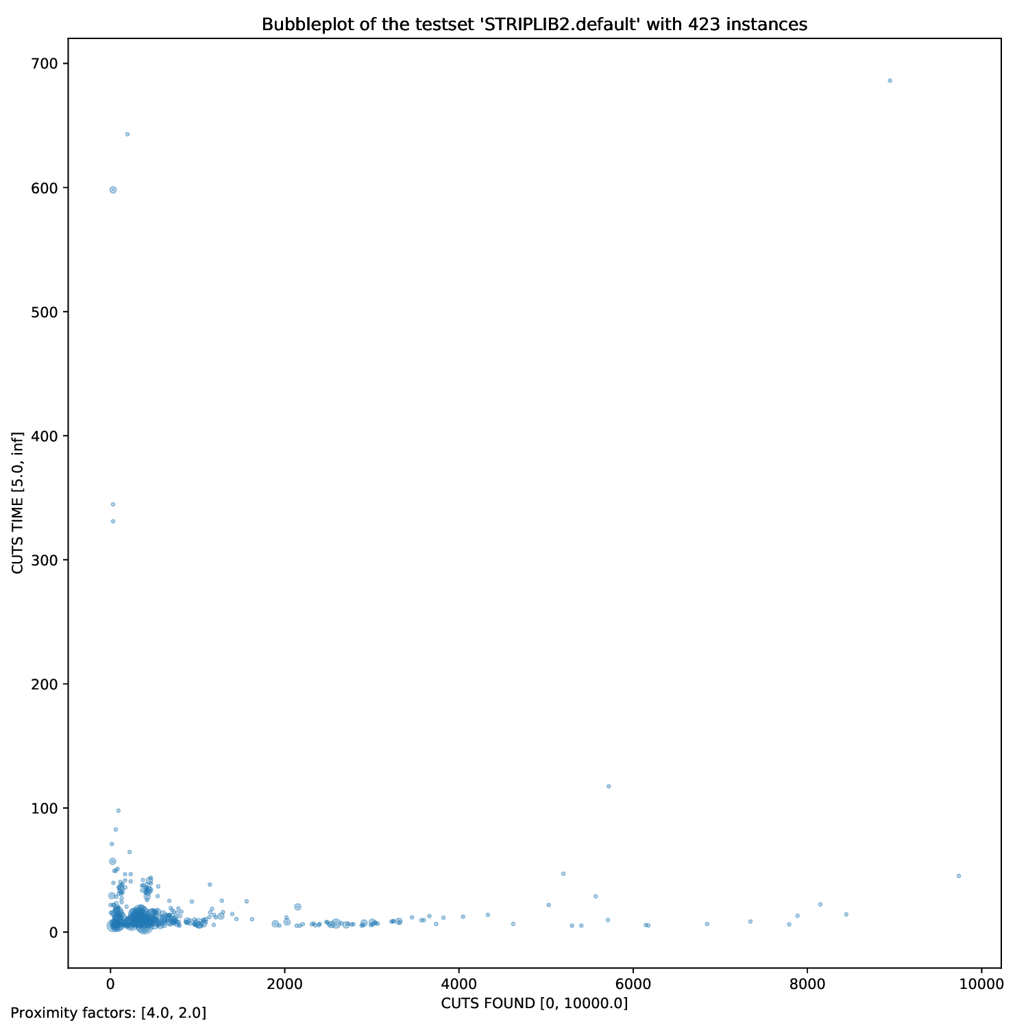
The general plotter is able to plot two or more arguments parsed by the general_parser.py script in different ways. You can find all parsed arguments here.
python3 general/{bubble,plot,twin,time}.py [args] FILES
with FILES being either some pickles, or some outfiles, and [args] being as defined below.
Times are the most common arguments to plot (that's the reason for the naming), but you can use whatever argument parsed you want. You can find a list of those here.
You can define what data to plot with the --times argument:
-t [TIMES [TIMES ...]], --times [TIMES [TIMES ...]]
                      times to be plotted.
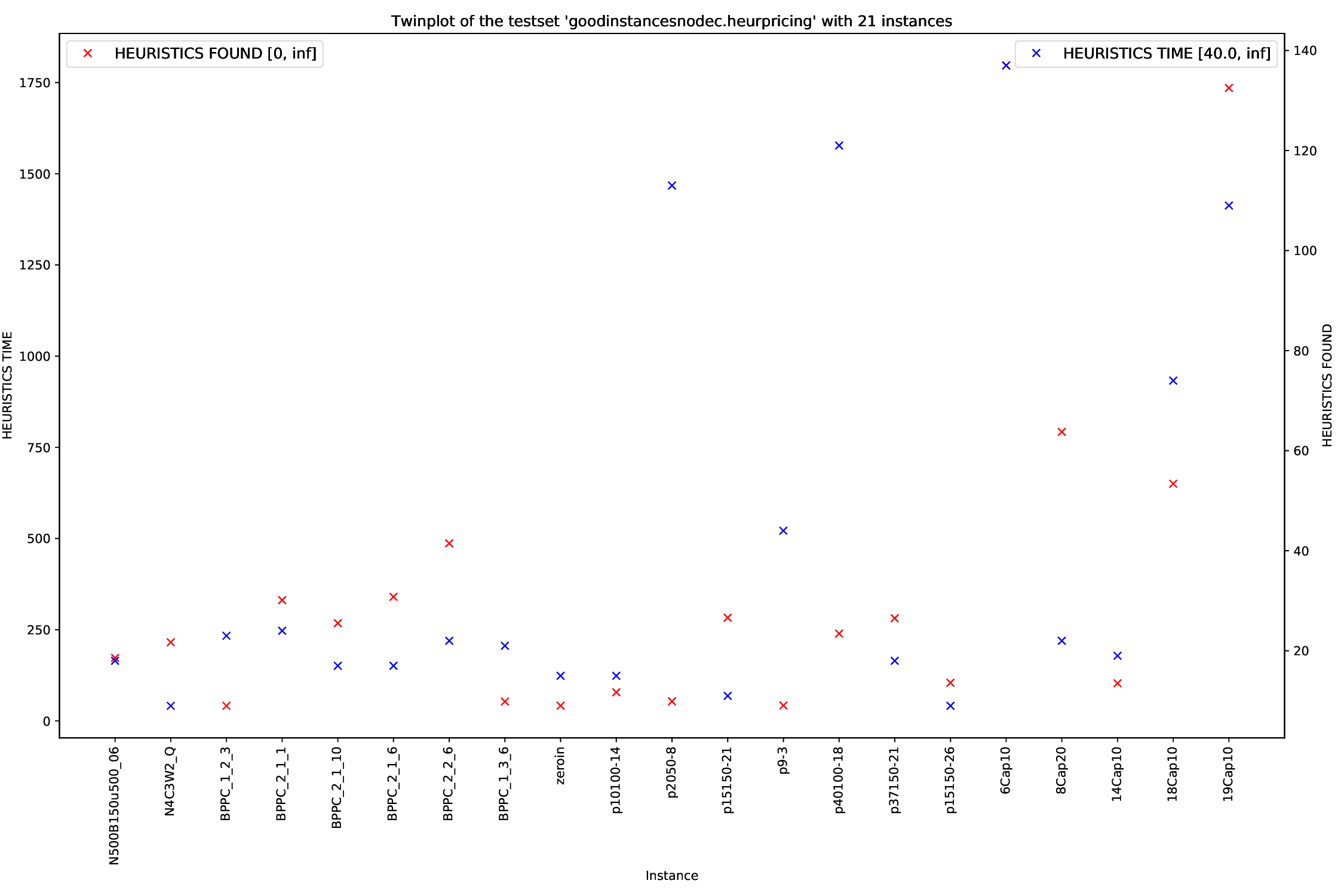
Whereas
bubble.py and twin.py, you may define exactly two times (or none), plot.py you can define as many times as you like andtime.py you can also define an arbitrary amount, but the "OTHERS" time will be added automatically.
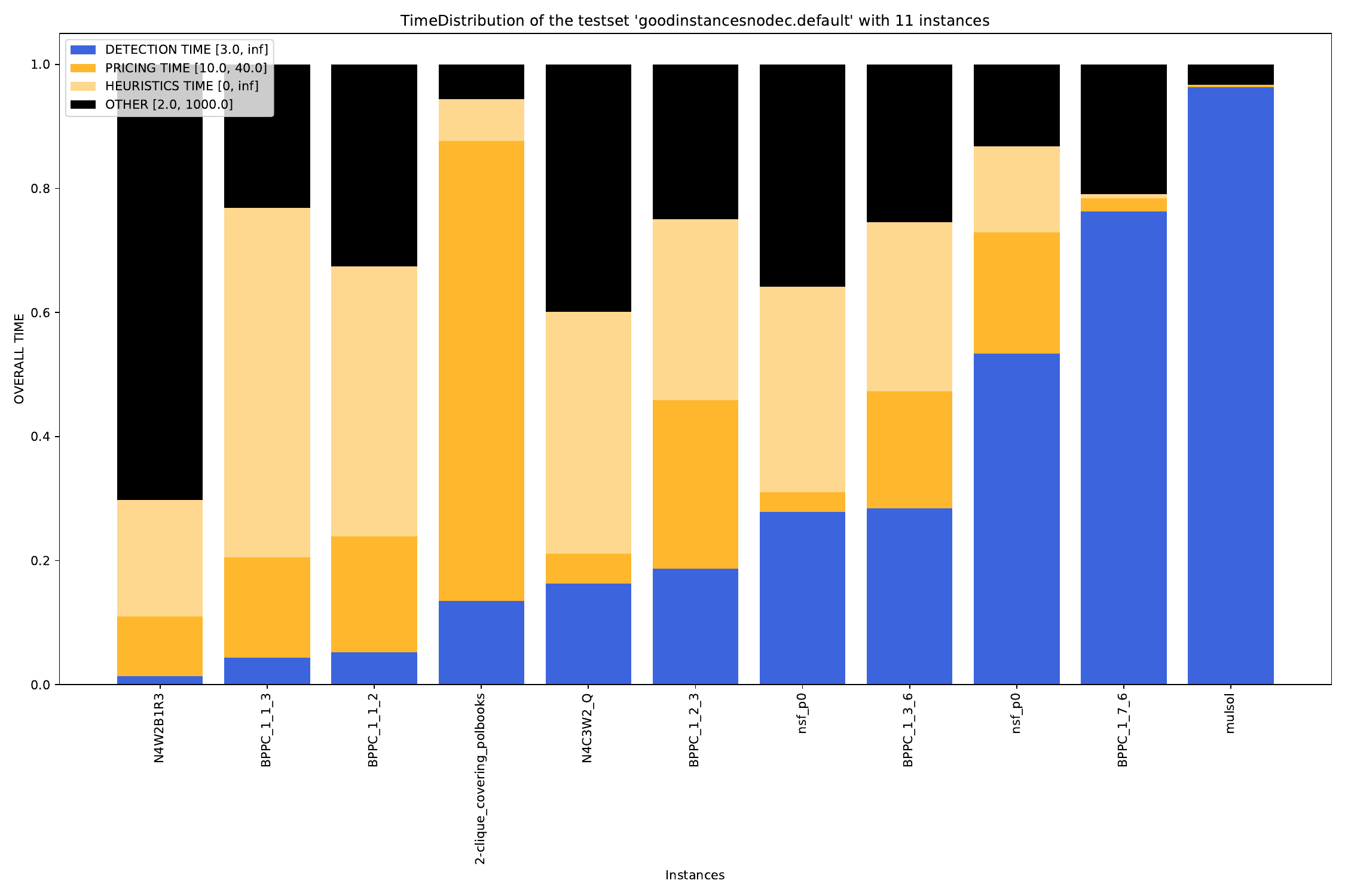
For all arguments, you can define filters. For example, if you only want to plot all those instances that had a Detection Time of between 10 and 20 seconds, you simply add those bounds to the time argument:
python3 general/time.py check.gcg.out -A -t "DETECTION TIME" 10 20 "RMP LP TIME"
In this example, we generate all plots (-A) for all instances that had a detection time between 10 and 20 seconds in the check.gcg.out file with the arguments "DETECTION TIME" and "RMP LP TIME" (without filter).
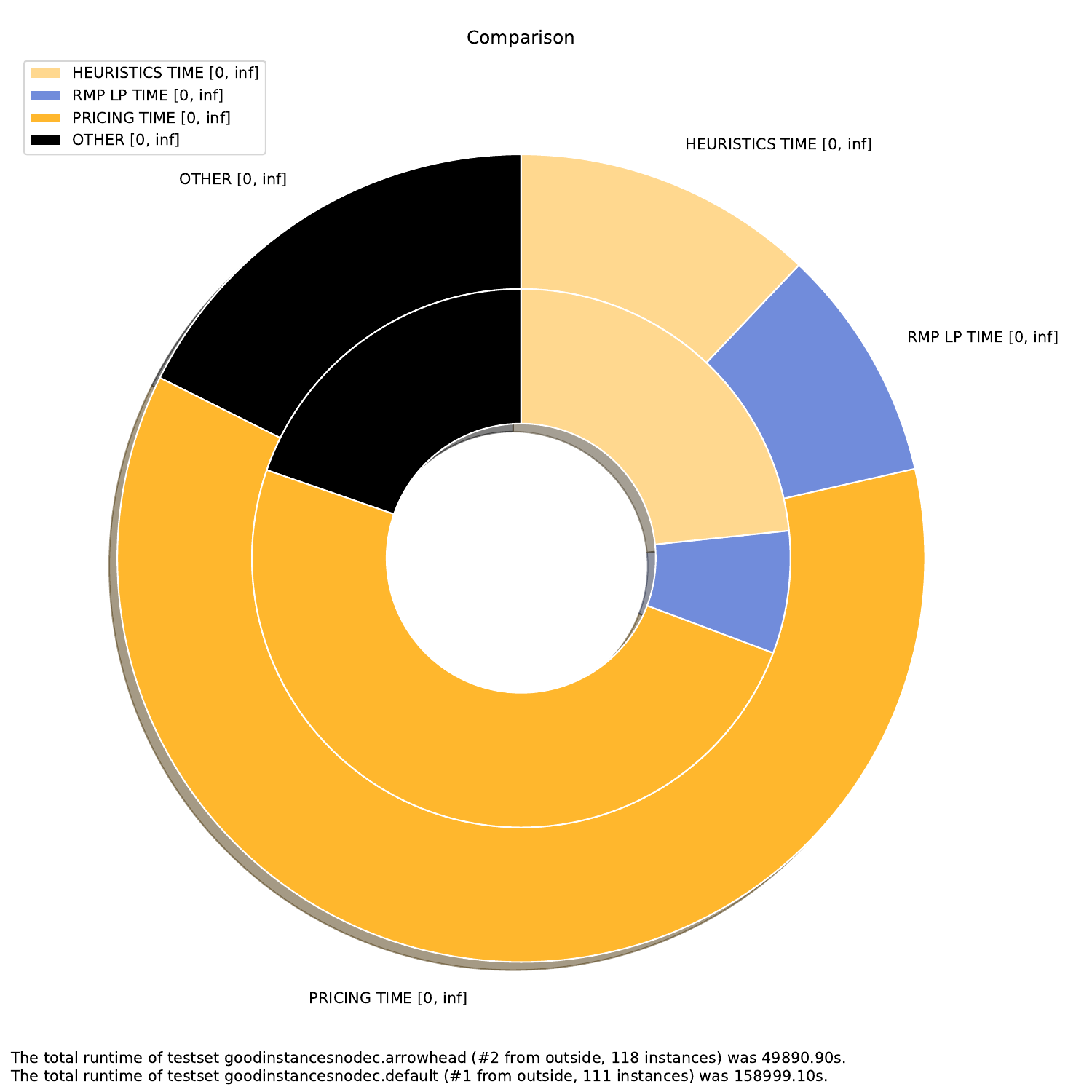
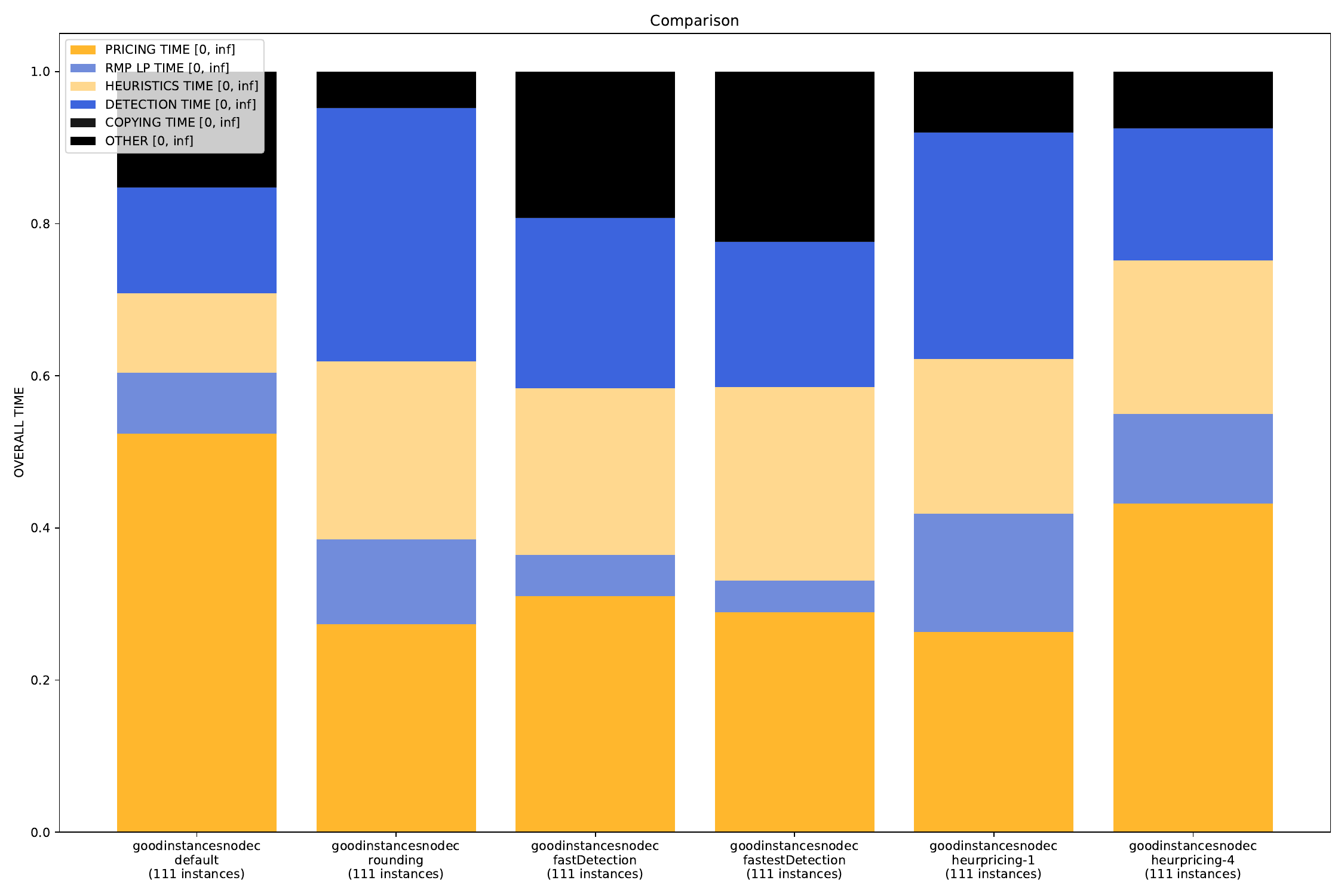
For the time.py script, you can define which plots you want to generate. The arguments are as follows:
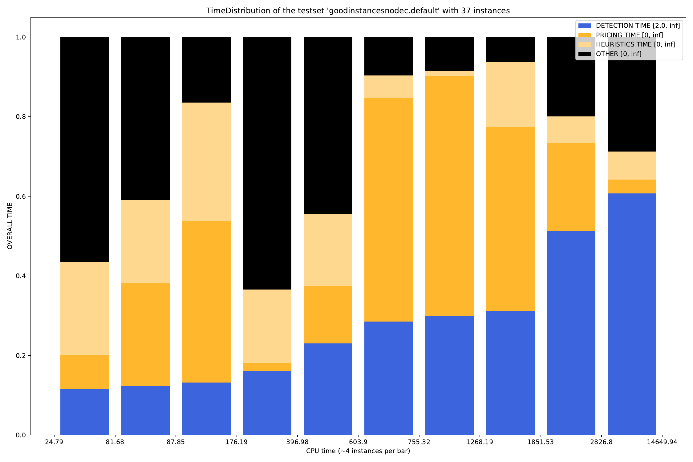
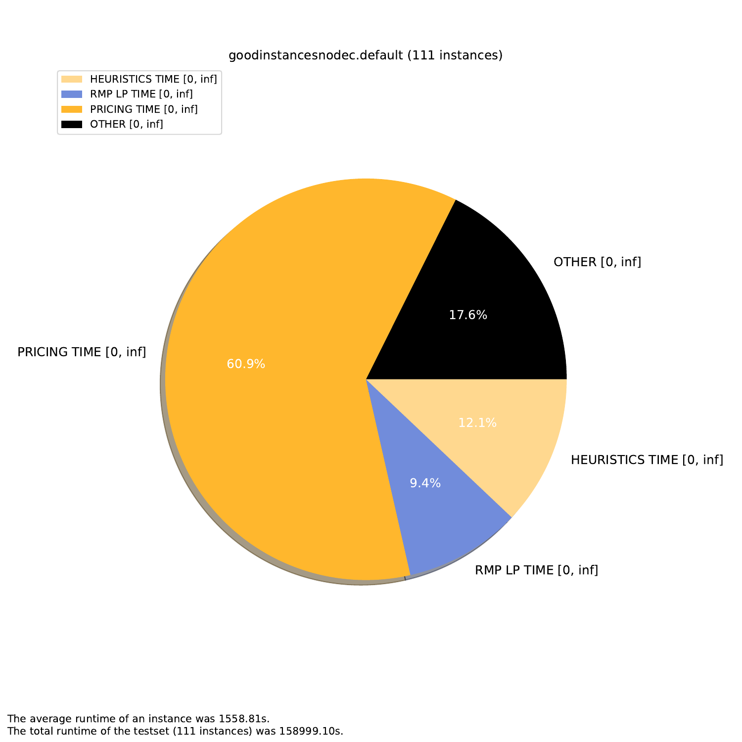
-A, --all             create all visualizations
-B, --bar             create barchart
-G, --grouped-bar     create barchart, grouped by CPU times
-P, --plot            create simple plot
--pie                 create a pie chart plot (will automatically activate --single (see below))
Additionally, for the grouped-bar plot, you may define a number of buckets, in which the script will automatically sort the (nearly) same number of instances into.
--buckets BUCKETS amount of buckets (resolution of grouped_bar plot)
Finally, you can compare two different runs. Though recommended, it is not required for the runs to have been on the same testset.
--single              if set, all outfiles will be summed and cumulated in a single plot
--compare             if set, each outfile will be summed and plotted with all other outfiles
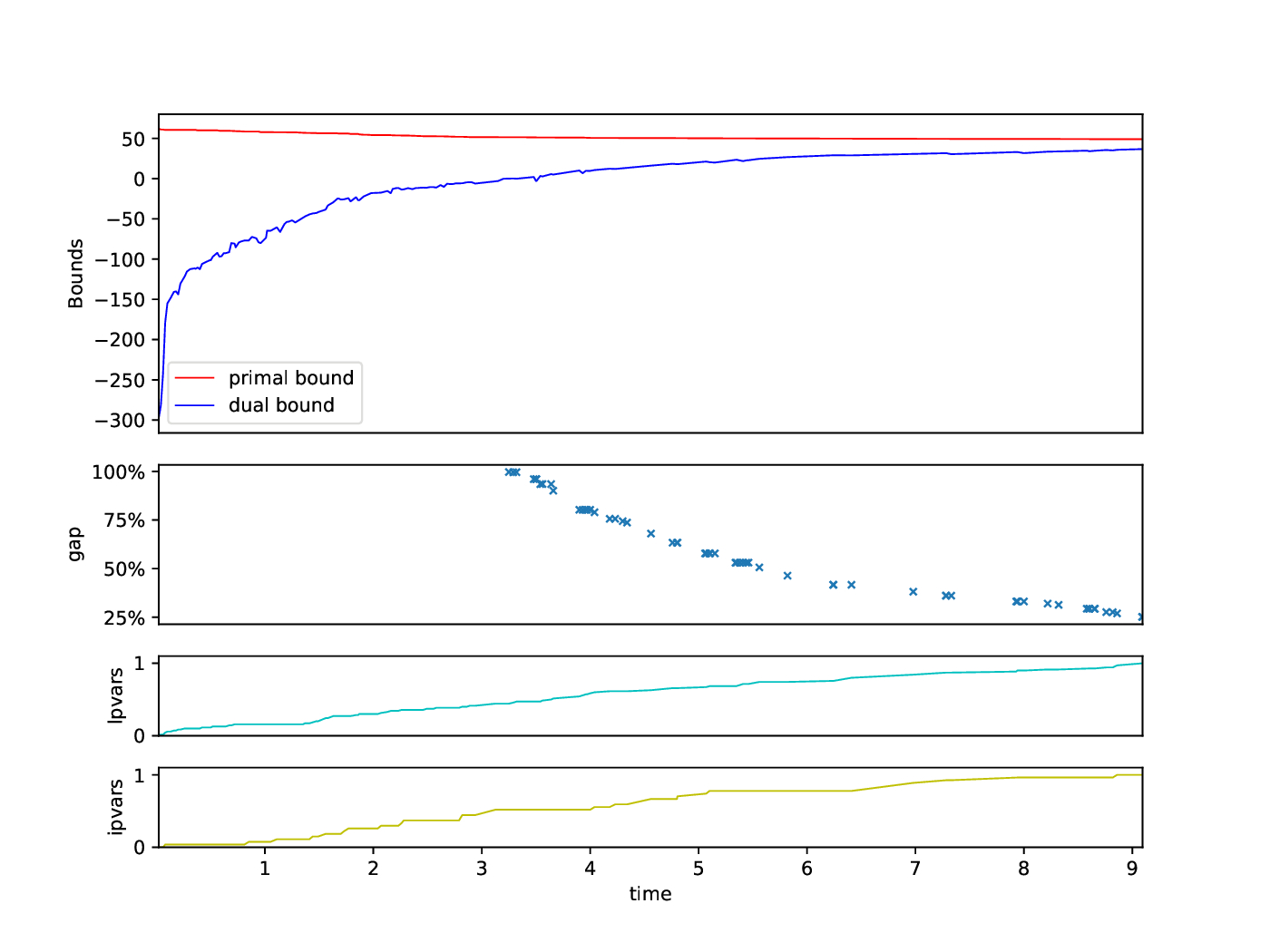
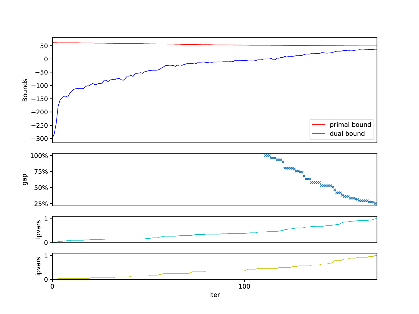
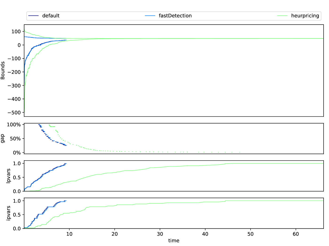
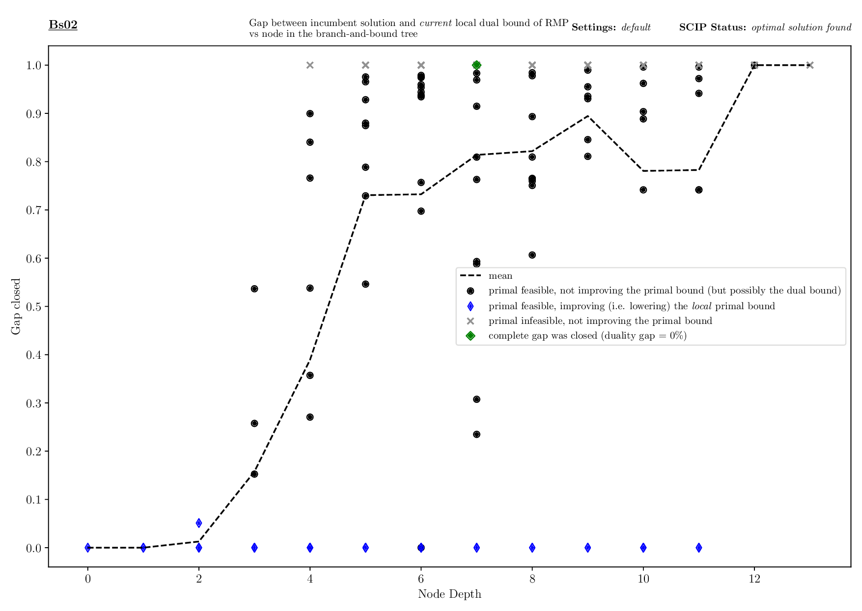
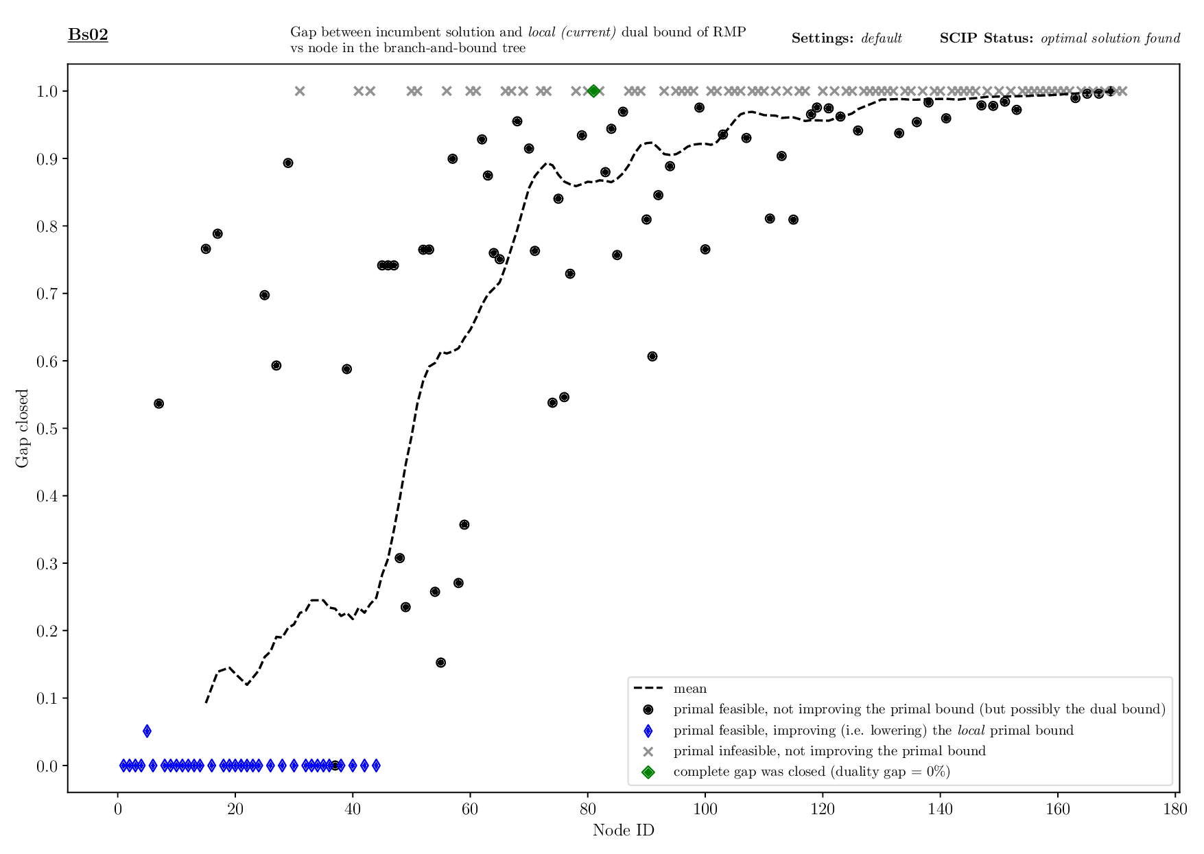
The Bounds Plotter generates a plot showing the development of the primal and dual bound and gap in the root node, as well as the basic variables generated.
python3 bounds/plotter_bounds.py FILES
with FILES being one or more .out files.
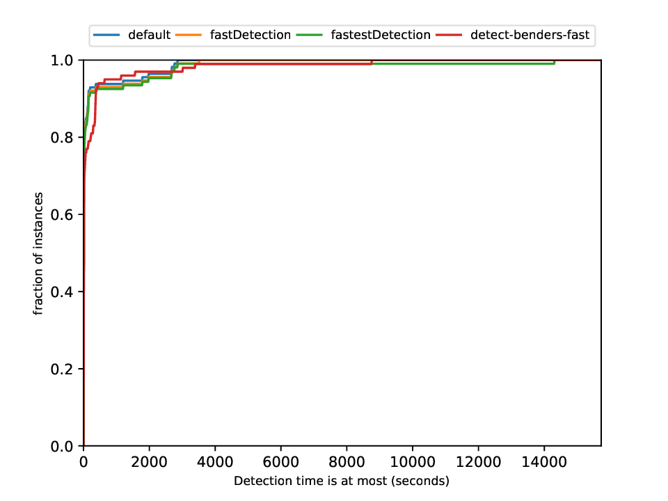
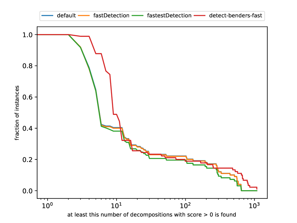
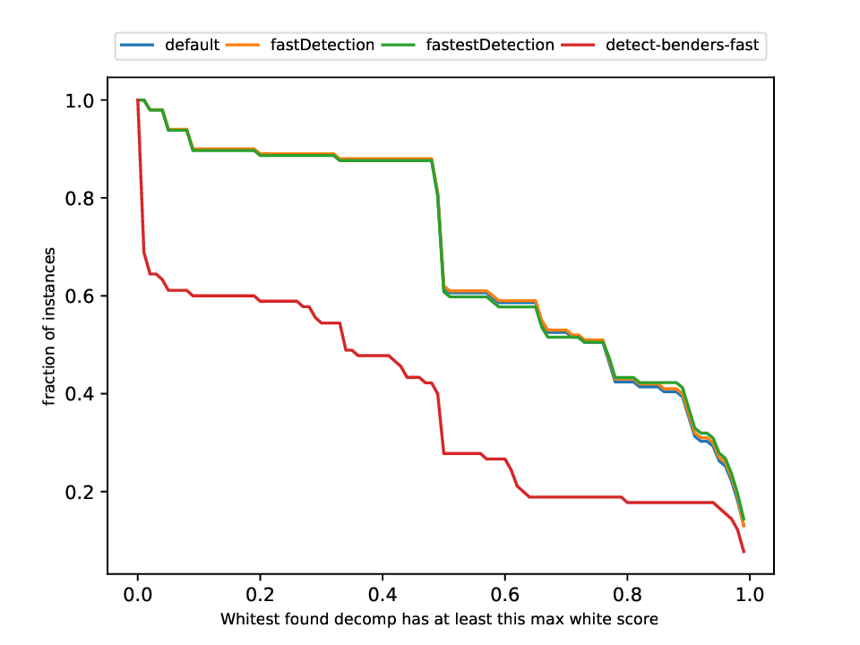
This plotter works on a whole testset and makes plots similar to performance profiles, showing the performance of the classifiers and detectors.
python3 detection/plotter_detection.py FILES
with FILES being one or more .out files.
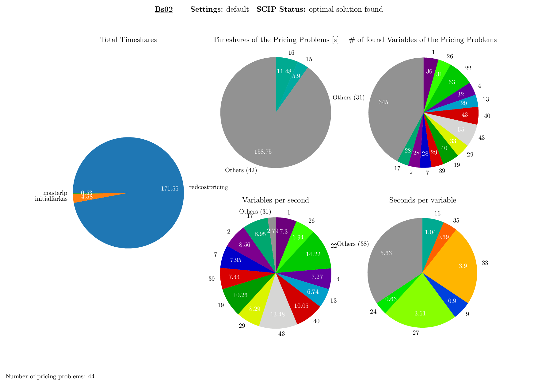
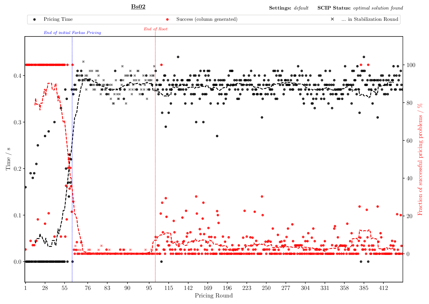
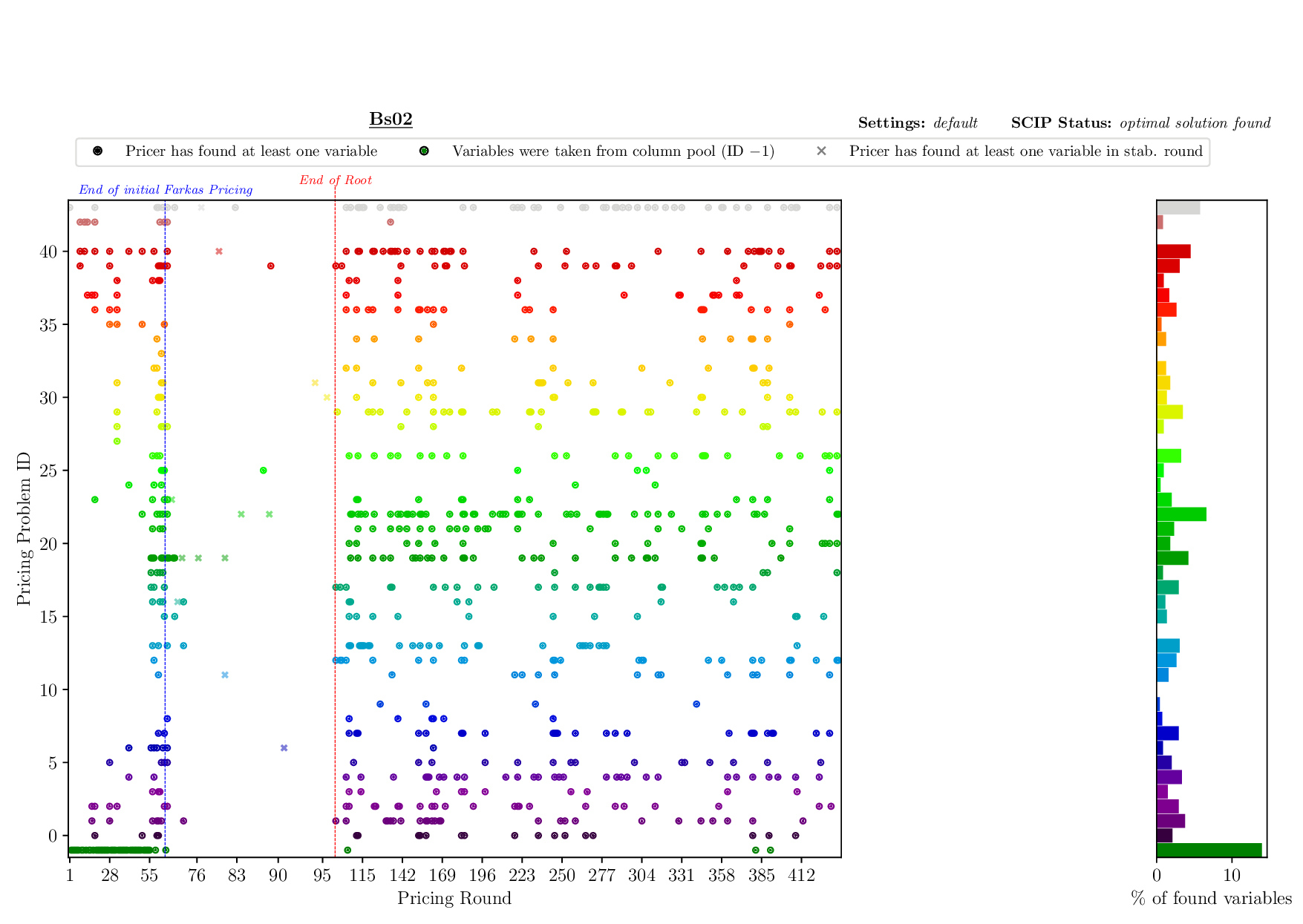
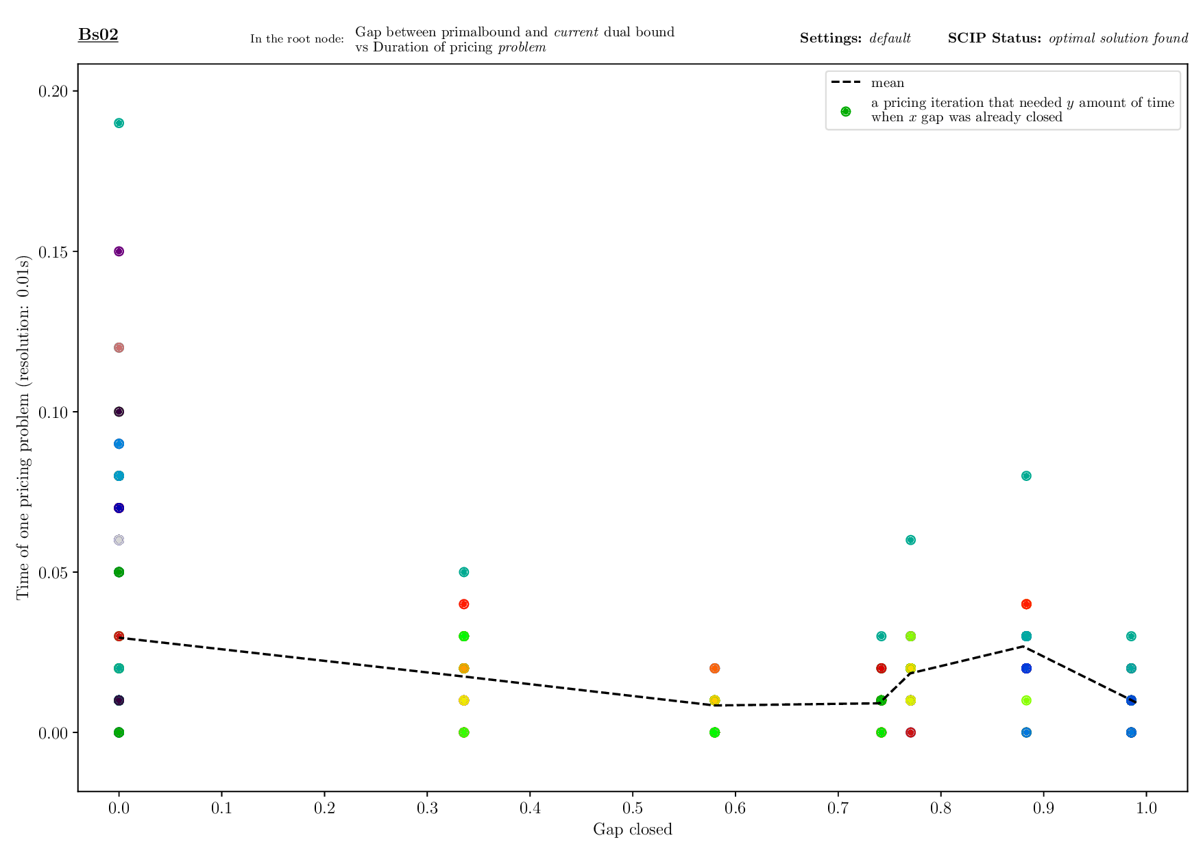
The Pricing Plotter generates 7 different plots illustrating the pricing procedure during a single instance's solving process. When given an outfile with more than one instance, it generates the plots sequentially.
python3 pricing/plotter_pricing.py FILES --vbcdir VBC
with FILES being one .out file and VBC being the directory where all corresponding .vbc files are (per default: check/results/vbc/)
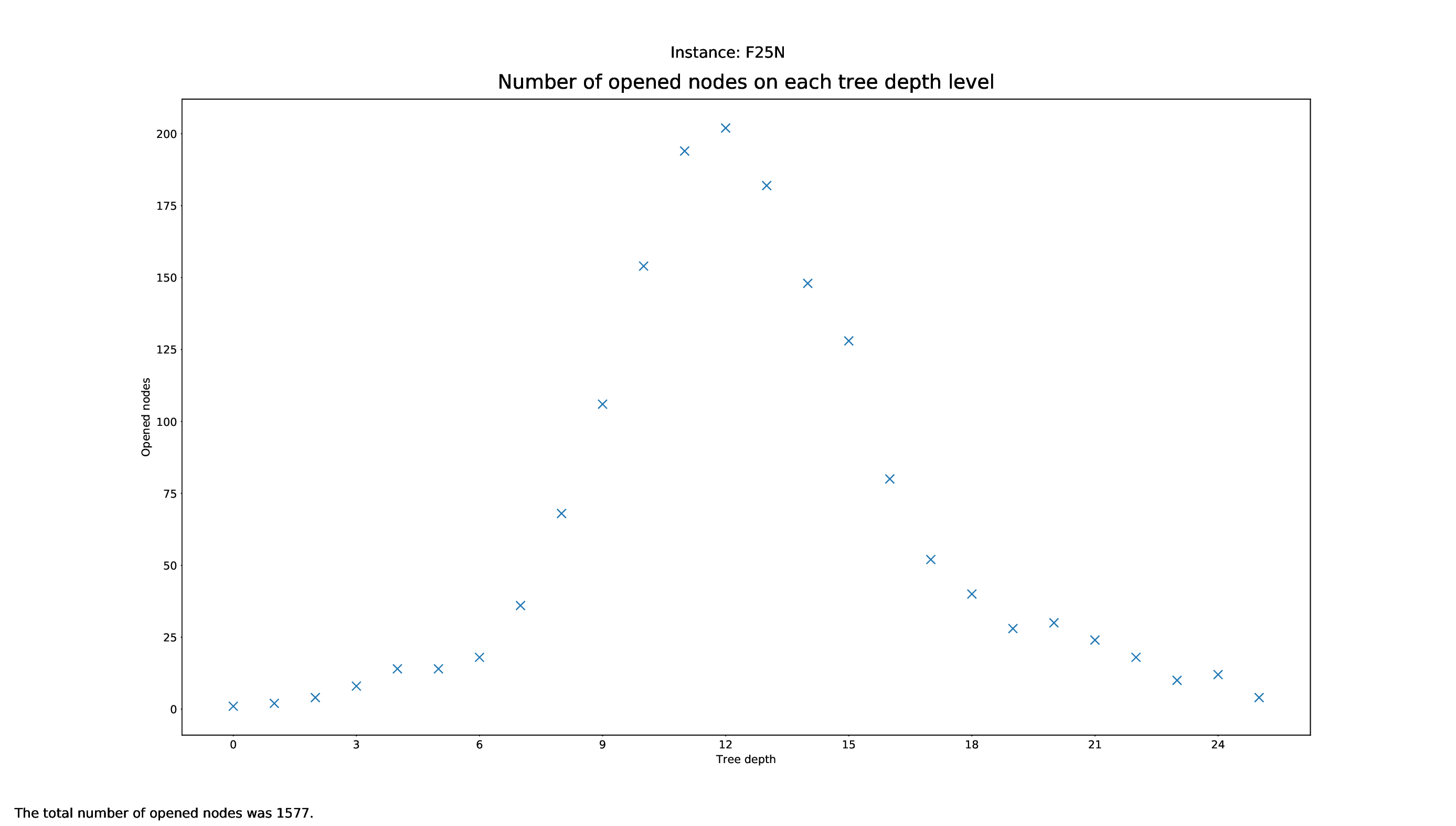
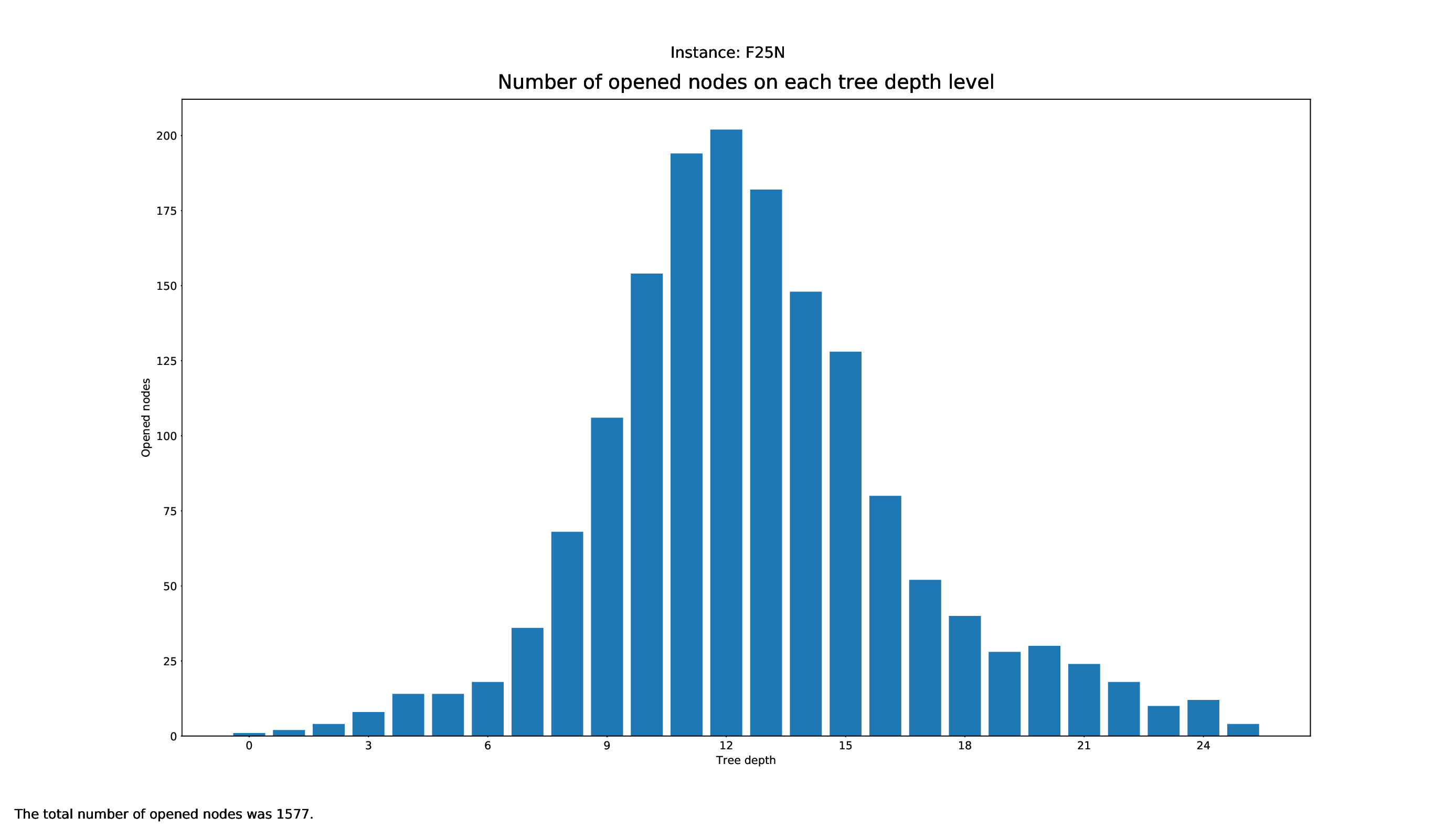
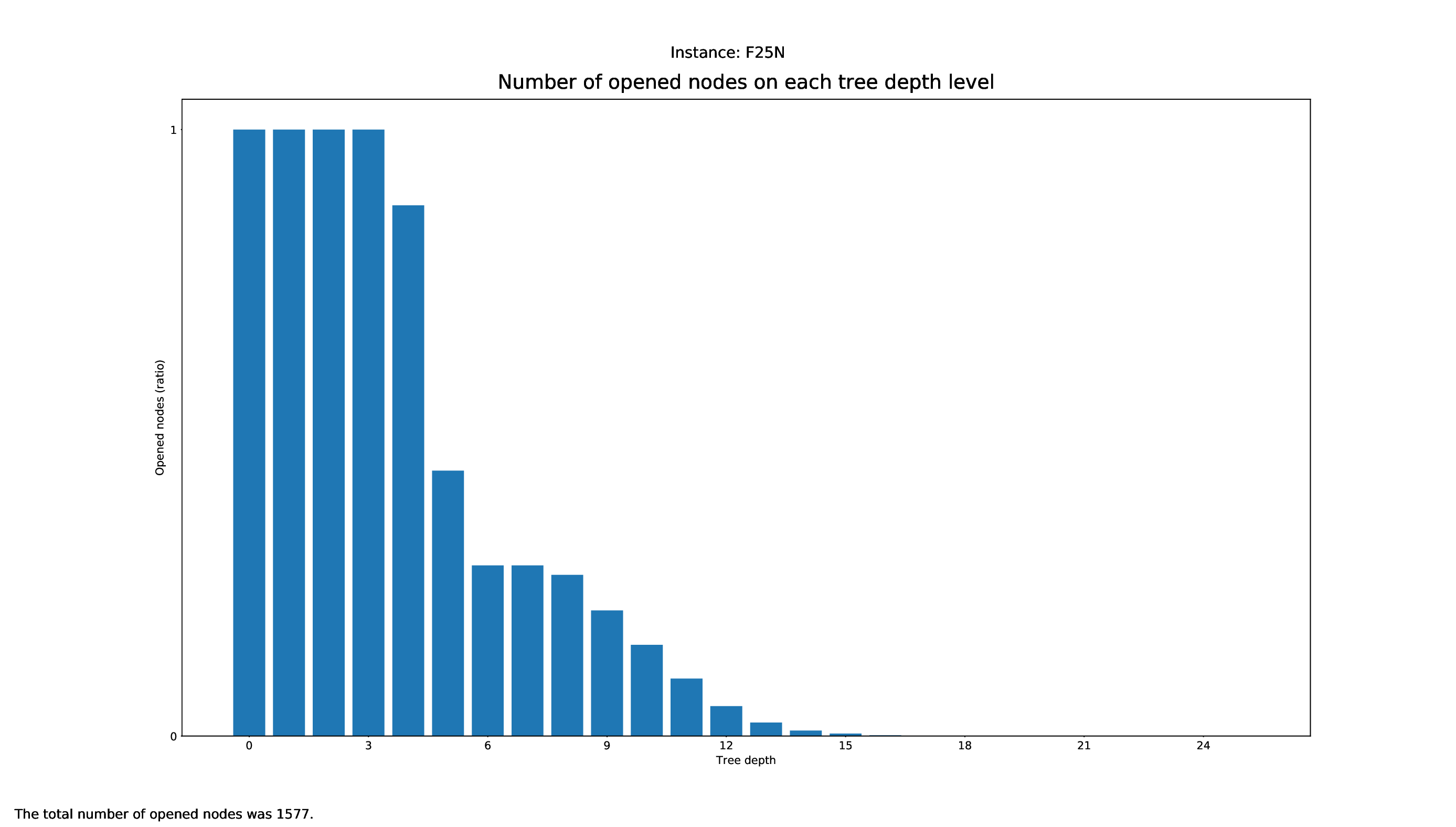
The Tree Statistics Plotter, just like the Pricing Plotter, needs the vbc files to function correctly. It will plot how many nodes were opened on each level.
python3 tree/plotter_tree.py FILES
with FILES being some .vbc files.
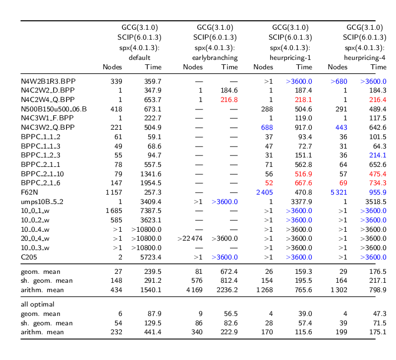
A (quite raw) comparison of testruns can be done using this script in the general-folder. This script just puts the statistics of all runs that are given as arguments into a .tex-file and prints it as ASCII on the console. Execution
./general/comparison_table.sh run1.res run2.res run3.res ...
with run1, run2, ... being a .res file in the format as shown in 'What files do I get'.
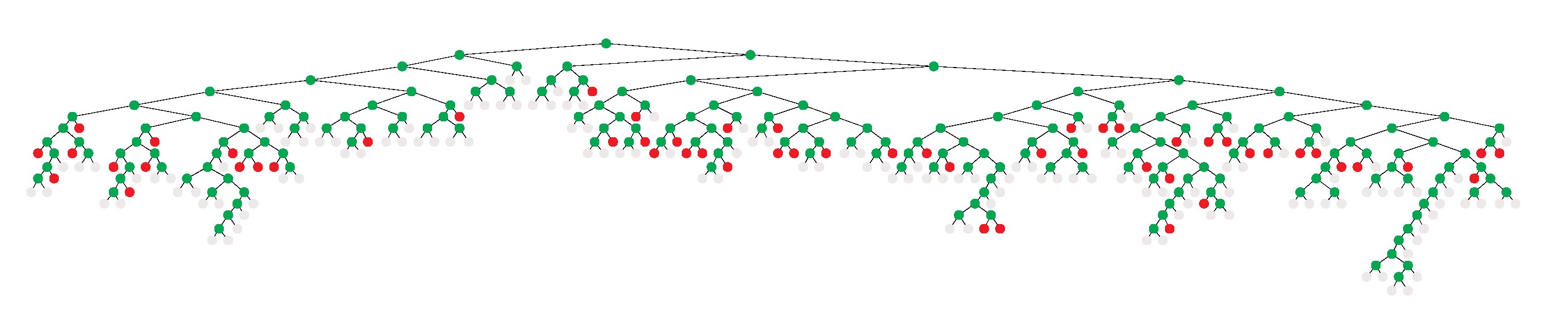
Note: The following guide concerns external software. We do not provide warranty nor support for it. Note: The tree visualization tool (vbctool) does not display aggregated information of the tree's development as the tree statistics plotter does, but shows the tree's development interactively.
In this section, we give a brief guide on how to use a tool to visualize branch-and-cut algorithmics, graphically showing how the tree was built during branching.
In order to generate pictures of the Branch and Bound tree that GCG used during solving, you can use the vbctool. Since the executable might have issues with the linking of the libraries, it is suggested to download the vbctool source code and additionally the Motif Framework source code, both available on the website. Unzip the Motif Framework source code tarball into the lib/ folder of the vbctool. Before starting with the Build Instructions, install the following packages:
sudo apt-get install libmotif-dev libxext-dev
Then, compile the program (just like explained in the Build Instructions):
cd lib/GFE
make
cd ../GraphInterface/
make
cd ../MotifApp/
make
cd ../..
make
Now you can start the program using
./vbctool
The files you now have to read (File -> Load) are included in the folder check/results/vbc.
In order to generate the tree, click on Emulation -> Start. Before doing that, you can configure the emulation in Emulation -> Setup, where you can also set the time it will need to generate the tree.
To save the generated tree, just click on File -> Print and it will save a .ps file.
Using existing runtime data, you can filter using the instructions under "General Plotter -> Arguments -> Defining Filters for the Data". For the strIPlib, we can provide a full data set (.out and .pkl format) of runtime data (which is also used in the strIPlib). To then export a test set including the instances that your filter applies to, you can set the flag -ts like that:
python3 general/plot.py check.gcg.out -ts -t "DETECTION TIME" 10 20 "RMP LP TIME"
Note that the test set file export mode is only implemented in the standard plotter, so please call plot.py with your filters and the test set export flag. After executing this command, you will get a test set file filtered.test in the given output directory, with which you can call the make test target as usual. If .dec files were used, they will be included in the exported test set file.
Whenever the test set that you get is too large to use or does not satisfy your requirements, we recommend to check out our diverse test set generation functionality.
When creating custom visualizations, one has to know exactly what data is needed to make the visualization. With these arguments in mind, one can then look if they are already parsed. A list of the currently parsed data is located here. If so, one of the parsers (parser_general.py, parser_bounds.py or parser_detection.py) can be used, or otherwise, for the plotter_pricing.py, the –savepickle argument of the plotter shall be used each time to parse the runtime data and save it to the pickle, to then read it again for the plotter. Then, the plotter_ script can be created which should import the parser that already gets the data needed with a simple import parser_.... Finally, the parser can be used just like in the other plotters.
Q: Why don't I get any detection times?
A: You probably did not run the test with a set mode, e.g. MODE=0, so GCG fell back to the readdec mode, reading any .dec files it could find instead of detecting.
 1.8.17