Creating and Solving Problems (e.g. with ZIMPL)

In this use case, we develop a branch-and-price algorithm for a combinatorial optimization problem without writing a single line of code. We only need to be able formulate our problem as a (mixed) integer program. For that we will use the ZIMPL modeling language.

The Problem

We consider a variant of a classic NP-hard combinatorial optimization problem. Given an undirected graph \(G=(V,E)\), a dominating set \(S\subseteq V\) is a subset of the vertices, such that every vertex \(i \in V\) is in \(S\) or adjacent to a vertex in \(S\). We say that every vertex not in \(S\) is dominated by a vertex in \(S\). For the capacitated dominating set problem we are additionally given vertex weights \(u:V\rightarrow \mathbb{Z}_+\). Loosely speaking, every vertex \(i \in V\) can dominate at most \(u(i)\) many other vertices. More formally, a subset \(S\subseteq V\) is a capacitated dominating set if and only if there exists a mapping \(f:V\setminus S\rightarrow S\) such that the number of vertices mapped under \(f\) to \(i\in S\) is no more than \(u(i)\).

The following example graph is taken from [5]. All vertices have capacity 2, and a minimum capacitated dominated set consists of e.g., \(S=\{2,6,7,8,12\}\). An arc \((i,j)\) is interpreted as '' \(i\) is dominated by \(j\),'' representing a possible mapping \(f\).

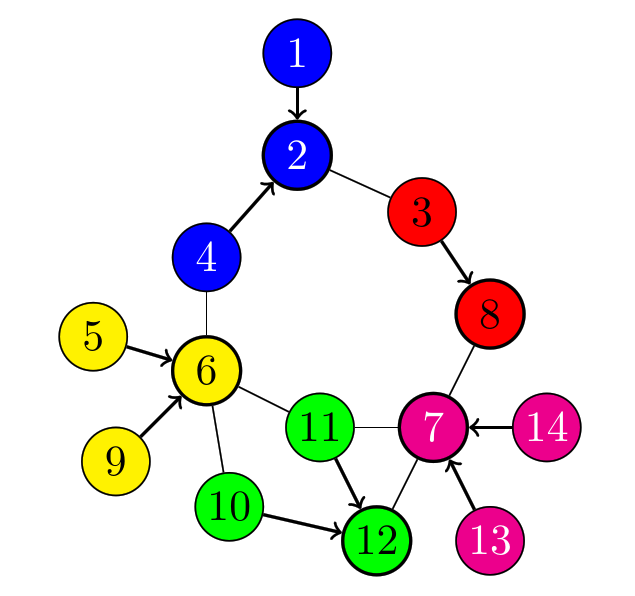
example graph where all vertices have capacity 2

A ''Textbook'' Binary Program

The following intuitive model was presented in [4] (actually, we corrected it a bit). We use variables \(x_i\in\{0,1\}\), \(i\in V\), to represent whether \(i\in S\), i.e., it is in the dominating set or not. The mapping \(f\) is represented by variables \(y_{ij}\in\{0,1\}\), \(\{i,j\}\in E\), that we interpret as \(y_{ij}=1 \iff f(j)=i\), that is, when \(i\) dominates \(i\). Define \(N(i):=\{j\in V : \{i,j\}\in E\}\) as the open neighborhood of \(i\in V\).

\begin{align} & \text{min} & & \sum_{i\in V}x_i \\ & \text{s.t.} & & \sum_{j\in N(i)} y_{ji} + x_i \geq 1 && i\in V \tag{BP} \\ & & & \sum_{j\in N(i)} y_{ij} \leq u_i x_i && i\in V \\ & & & x_i\in\{0,1\} && i\in V \\ & & & y_{ij}\in\{0,1\} && \{i,j\}\in E \end{align}

The objective function minimizes \(|S|\). Every vertex has to be dominated by a neighbor or is itself in \(S\); and no vertex can dominate more vertices than given by its capacity (the capacity is available only if the vertex is in \(S\)). Thus, the capacity constraints also link the \(x\) and \(y\) variables.

A ZIMPL model file (download) for the above instance is as follows:

# vertices
set V := {1 .. 14};
# (undirected) edges
set E := {<1,2>, <2,3>, <2,4>, <4,6>, <3,8>, <7,8>, <5,6>, <6,9>, <6,10>, <6,11>, <7,11>, <7,12>, <7,13>, <7,14>, <10,12>, <11,12>};
# (directed) arcs, produced from (undirected) edges
set A := E union {<j,i> in V*V with <i,j> in E};
 
# uniform capacity of 2 for each vertex
param cap[<v> in V] := 2;
 
# neighbors of v
defset N(v) := {<i> in V with <v,i> in A};
 
 
# is v selected in the dominating set?
var x[V] binary;
 
# for <i,j> in A: is j dominated by i?
var y[A] binary;
 
 
minimize cost: sum<v> in V: x[v];
 
# every vertex v must be dominated by some vertex i (unless v is selected)
subto dominate:
        forall <v> in V: sum<i> in N(v): y[i,v] + x[v] >= 1;
 
# the domination capacity of each vertex must be respected
subto capacity:
        forall <v> in V: sum<i> in N(v): y[v,i] <= x[v]*cap[v];

Of course, you can use any modeling language you like, or generate your model (typically in .lp or .mps format) using a script. A bonus from using ZIMPL is that GCG can directly read the model file (when you compiled it with ZIMPL=true). So, we start GCG and

GCG> read potluri+singh.zpl
 
...
 
original problem has 46 variables (46 bin, 0 int, 0 impl, 0 cont) and 28 constraints
GCG>

If GCG complains about a missing reader (because you compiled it with ZIMPL=false), alternatively run ZIMPL on the .zpl file to generate an .lp or .mps, and read this into GCG. Then start the optimization.

GCG> optimize
 
...
 
A Dantzig-Wolfe reformulation is applied to solve the original problem.
 
  time | node  | left  |SLP iter|MLP iter|LP it/n| mem |mdpt |ovars|mvars|ocons|mcons|mcuts|  dualbound   | primalbound  |  deg   |  gap   
t  0.0s|     1 |     0 |      0 |      0 |     - | 905k|   0 |  17 |   0 |   9 |   0 |   0 | 3.000000e+00 | 1.200000e+01 |   --   | 300.00%
i  0.0s|     1 |     0 |      0 |      0 |     - | 915k|   0 |  17 |   0 |   9 |   0 |   0 | 3.000000e+00 | 8.000000e+00 |   --   | 166.67%
*  0.0s|     1 |     0 |      0 |      0 |     - | 915k|   0 |  17 |   0 |   9 |   0 |   0 | 5.000000e+00 | 5.000000e+00 |   --   |   0.00%
   0.0s|     1 |     0 |      0 |      0 |     - | 915k|   0 |  17 |   0 |   9 |   0 |   0 | 5.000000e+00 | 5.000000e+00 |   --   |   0.00%
 
SCIP Status        : problem is solved [optimal solution found]
Solving Time (sec) : 0.01
Solving Nodes      : 1
Primal Bound       : +5.00000000000000e+00 (4 solutions)
Dual Bound         : +5.00000000000000e+00
Gap                : 0.00 %
 
GCG>

When we look at the optimal solution we find \(S=\{2,6,7,8,12\}\) as in the figure above.

GCG> display solution
 
objective value:                                    5
x#2                                                 1   (obj:1)
x#6                                                 1   (obj:1)
x#7                                                 1   (obj:1)
x#8                                                 1   (obj:1)
x#12                                                1   (obj:1)
y#2#4                                               1   (obj:0)
y#2#1                                               1   (obj:0)
y#7#13                                              1   (obj:0)
y#7#14                                              1   (obj:0)
y#6#9                                               1   (obj:0)
y#6#5                                               1   (obj:0)
y#8#3                                               1   (obj:0)
y#8#7                                               1   (obj:0)
y#12#11                                             1   (obj:0)
y#12#10                                             1   (obj:0)
 
GCG>

This instance is too easy, so not much happens in GCG (in particular no branching). But when we try a larger instance (like this one with 250 vertices, 3780 edges, and uniform capacities of 5 for each vertex; taken from [5]), we witness a full-fledged branch-and-price algorithm at work to solve the capacitated dominating set problem:

GCG> read uni-UDG-5-250-150-graphS0N250.mps.gz
 
...
 
original problem has 4030 variables (0 bin, 4030 int, 0 impl, 0 cont) and 500 constraints
GCG> optimize
 
...
 
A Dantzig-Wolfe reformulation is applied to solve the original problem.
 
  time | node  | left  |SLP iter|MLP iter|LP it/n| mem |mdpt |ovars|mvars|ocons|mcons|mcuts|  dualbound   | primalbound  |  deg   |  gap   
p  0.1s|     1 |     0 |      0 |      0 |     - |  19M|   0 |4011 |   0 | 494 |   0 |   0 | 1.000000e+00 | 2.460000e+02 |   --   |  Large
   0.2s|     1 |     0 |      0 |      0 |     - |  18M|   0 |4011 |   0 | 494 |   0 |   0 | 4.250000e+01 | 2.460000e+02 |   --   | 478.82%
r  0.2s|     1 |     0 |      0 |      0 |     - |  18M|   0 |4011 |   0 | 494 |   0 |   0 | 4.250000e+01 | 1.180000e+02 |   --   | 177.65%
Chosen structure has 245 blocks, 3 master-only (static) variables, and 249 linking constraints.
This decomposition has a maxwhite score of 0.493929.
Master problem is a set covering problem.
Matrix has 245 blocks, using 245 pricing problems.
 
 
   0.8s|     1 |     0 |      0 |      0 |     - |  93M|   0 |4011 | 248 | 495 | 495 |   0 | 4.250000e+01 | 1.180000e+02 |   0.00%| 177.65%
   0.8s|     1 |     0 |      0 |      0 |     - |  94M|   0 |4011 | 493 | 495 | 495 |   0 | 4.250000e+01 | 1.180000e+02 |   0.00%| 177.65%
Starting reduced cost pricing...
*r 0.8s|     1 |     0 |    522 |    522 |     - |  95M|   0 |4011 | 619 | 495 | 495 |   0 | 4.250000e+01 | 1.160000e+02 |  20.26%| 172.94%
   0.8s|     1 |     0 |    522 |    522 |     - |  95M|   0 |4011 | 619 | 495 | 495 |   0 | 4.250000e+01 | 1.160000e+02 |  20.26%| 172.94%
*r 0.8s|     1 |     0 |    591 |    591 |     - |  95M|   0 |4011 | 667 | 495 | 495 |   0 | 4.250000e+01 | 1.120000e+02 |  21.67%| 163.53%
   0.8s|     1 |     0 |    591 |    591 |     - |  95M|   0 |4011 | 667 | 495 | 495 |   0 | 4.250000e+01 | 1.120000e+02 |  21.67%| 163.53%
*r 0.8s|     1 |     0 |    594 |    594 |     - |  95M|   0 |4011 | 668 | 495 | 495 |   0 | 4.250000e+01 | 1.110000e+02 |  22.12%| 161.18%
   0.8s|     1 |     0 |    594 |    594 |     - |  95M|   0 |4011 | 668 | 495 | 495 |   0 | 4.250000e+01 | 1.110000e+02 |  22.12%| 161.18%
   1.0s|     1 |     0 |   4657 |   4657 |     - |  96M|   0 |4011 |1370 | 495 | 495 |   0 | 4.250000e+01 | 1.110000e+02 |  12.46%| 161.18%
*r 1.0s|     1 |     0 |   4657 |   4657 |     - |  97M|   0 |4011 |1370 | 495 | 495 |   0 | 4.250000e+01 | 1.100000e+02 |  12.46%| 158.82%
   1.0s|     1 |     0 |   4657 |   4657 |     - |  97M|   0 |4011 |1370 | 495 | 495 |   0 | 4.250000e+01 | 1.100000e+02 |  12.46%| 158.82%
*o 1.1s|     1 |     0 |   6042 |   6042 |     - |  97M|   0 |4011 |1370 | 495 | 495 |   0 | 4.250000e+01 | 5.000000e+01 |  12.46%|  17.65%
  time | node  | left  |SLP iter|MLP iter|LP it/n| mem |mdpt |ovars|mvars|ocons|mcons|mcuts|  dualbound   | primalbound  |  deg   |  gap   
   1.1s|     1 |     0 |   6042 |   6042 |     - |  97M|   0 |4011 |1370 | 495 | 495 |   0 | 4.250000e+01 | 5.000000e+01 |  12.46%|  17.65%
   2.0s|     1 |     2 |   6042 |   6042 |     - | 118M|   0 |4011 |2595 | 495 | 495 |   0 | 4.250000e+01 | 5.000000e+01 |  12.46%|  17.65%
*r 5.0s|    85 |    84 |  41737 |  41737 | 424.9 | 124M|  84 |4011 |4840 | 495 | 495 |   0 | 4.250000e+01 | 4.900000e+01 |   --   |  15.29%
   5.5s|   100 |   101 |  44907 |  44907 | 392.6 | 125M|  99 |4011 |5240 | 495 | 495 |   0 | 4.250000e+01 | 4.900000e+01 |   --   |  15.29%
*r 5.9s|   111 |   110 |  48242 |  48242 | 383.6 | 127M| 110 |4011 |5740 | 495 | 495 |   0 | 4.250000e+01 | 4.800000e+01 |   --   |  12.94%
*r 6.3s|   127 |   126 |  50109 |  50109 | 349.7 | 128M| 126 |4011 |6190 | 495 | 495 |   0 | 4.250000e+01 | 4.700000e+01 |   --   |  10.59%
*r 6.4s|   128 |   127 |  50283 |  50283 | 348.4 | 129M| 127 |4011 |6267 | 495 | 495 |   0 | 4.250000e+01 | 4.600000e+01 |   --   |   8.24%
*r 6.4s|   130 |   129 |  50337 |  50337 | 343.4 | 129M| 129 |4011 |6267 | 495 | 495 |   0 | 4.250000e+01 | 4.500000e+01 |   --   |   5.88%
  12.2s|   200 |   187 |  84603 |  84603 | 394.8 | 131M| 149 |4011 |7062 | 495 | 495 |   0 | 4.250000e+01 | 4.500000e+01 |   --   |   5.88%
  19.5s|   300 |   285 | 119930 | 119930 | 380.9 | 138M| 149 |4011 |9374 | 495 | 495 |   0 | 4.250000e+01 | 4.500000e+01 |   --   |   5.88%
*L23.5s|   330 |   290 | 136161 | 136161 | 395.5 | 139M| 149 |4011 |9474 | 495 | 495 |   0 | 4.250000e+01 | 4.400000e+01 |   --   |   3.53%
  29.0s|   400 |   360 | 164359 | 164359 | 396.8 | 143M| 149 |4011 |  11k| 495 | 495 |   0 | 4.250000e+01 | 4.400000e+01 |   --   |   3.53%
*r29.8s|   412 |     0 | 166163 | 166163 | 389.6 | 144M| 149 |4011 |  11k| 495 | 495 |   0 | 4.266667e+01 | 4.300000e+01 |   --   |   0.78%
 
SCIP Status        : problem is solved [optimal solution found]
Solving Time (sec) : 29.81
Solving Nodes      : 412
Primal Bound       : +4.30000000000000e+01 (26 solutions)
Dual Bound         : +4.30000000000000e+01
Gap                : 0.00 %
 
GCG>

GCG applied a Dantzig-Wolfe reformulation of the (''original'') input model to obtain an equivalent (''master'') integer program. The latter is solved by branch-and-price, that is, the linear relaxation in each node of the branch-and-bound tree is solved by column generation. GCG automatically detects what subproblems to form from the original problem.

We could stop here because our problem is solved. However, when you already know some theory about branch-and-price and Dantzig-Wolfe reformulation, we can provide you with some background and ways to influence the solution process.

A Binary Program Based on Subsets of Vertices

In the compact model, the \(y\)-variables represent subsets \(T_i := \{j \in V : y_{ij}=1\} \subseteq N(i)\) of neighbors, for each vertex \(i\in V\). The important observation is that an (optimal) solution \(S\) to the capacitated dominated set problem corresponds to a partition of the vertices into (a minimum number of) subsets \(T_i \cup \{i\}\), one for each vertex \(i\in S\). The color classes in the figure above exactly reflect these vertex subsets.

We base an alternative model on this observation: Introduce a binary variable \(\lambda^i_T\in\{0,1\}\) for each possible subset \(T\subseteq N(i) \cup \{i\}\) of neighbors of \(i\in V\) (and \(i\) itself), where we require \(i\in T\) and \(|T|\leq u_i+1\). Denote by \({\cal T}_i\) the collection of all such vertex subsets for \(i\in V\). We then state a set partitioning model:

\begin{align} & \text{min} & & \sum_{i\in V}\sum_{T \in {\cal T}_i} \lambda^i_T \\ & \text{s.t.} & & \sum_{j\in N(i)}\sum_{T \in {\cal T}_j : i \in T} \lambda^j_T = 1 && i\in V & [\alpha_i] \tag{MP}\\ & & & \sum_{T \in {\cal T}_i} \lambda^i_T \leq 1 && i\in V & [\beta_i]\\ & & & \lambda^i_T\in\{0,1\} && i\in V,\, T\in {\cal T}_i \\ \end{align}

The objective is to miminimize the cardinality of the partition. Each vertex must appear in exactly one selected vertex subset and no more than one subset can be selected per vertex (could be none). In brackets, we indicate the dual variables per constraint. The cardinality of \({\cal T}_i\) is \(|N(i)| \choose u_i\), which in general can be exponential in \(|V|\). This suggests to solve the linear relaxation by column generation. The restricted master problem (RMP) contains only a (small) subset \({\cal T}'_i \subseteq {\cal T}_i\) for each \(i\in V\), initially, say, \({\cal T}'_i=\{\{i\}\}\). This initialization corresponds to the worst possible solution that every vertex is in the dominating set, but technically, this ensures feasibility of the RMP.

In order to determine a \(\lambda^i_T\) variable with \(T\in {\cal T}_i \setminus {\cal T}'_i\) of negative reduced cost (or to prove that none exists), we solve a pricing problem for each \(i\in V\). It reads as

\begin{align} z := \enspace & \text{min} & & 1 - \sum_{j\in N(i)} \alpha_j y_j - \alpha_i - \beta_i\\ & \text{s.t.} & & \sum_{j\in N(i)} y_j \leq u_i \tag{PP} \\ & & & y_j\in\{0,1\} && j\in V \end{align}

Note again that in this model, \(i\in V\) is fixed. As a solution, a capacitated subset \(T=\{j\in N(i) : y_j=1\} \cup \{i\}\) of neighbors of \(i\in V\) (and \(i\) itself) is selected. The objective function minimizes the reduced cost of the corresponding \(\lambda\)-variable (assuming again that \(i\in T\)).

When \(z<0\), variable \(\lambda^i_T\) is added to the RMP; the RMP is re-optimized, new dual variable values are obtained, and the process iterates. Otherwise, i.e., \(z\geq0\), we have proven optimality of the the linear relaxation of the master problem, and we can branch. As the master problem is a set partitioning problem, Ryan-Foster branching [6] is a good choice.

Dantzig-Wolfe Reformulation

work in progress below this point

Actually, this alternative model results from a Dantzig-Wolfe reformulation of the compact model.

GCG by default does not make use of the row and column names, but it can be told to do so:

GCG> set detection consclassifier consnamenonumbers origenabled TRUE

decomposition with 14 blocks

decomposition with 14 blocks and linking variables

If you are interested, Potluri and Singh [5] made all their instances publicly available for download, together with the C code for their heuristics. We provide ZIMPL model files that read their input, for uniform and [variable](todo) capacities.

The authors .. provide the data they used in their publication [here] and a general ZIMPL that can read their instances as input is [here (local ressource)].

old

We would like to answer two questions:

What exactly happened? (alternative model and Dantzig-Wolfe reformulation)
Is it worth it? (is this faster than SCIP?)

was it worth it?

compare SCIP on the original model, GCG with our selected decomposition, and GCG automatic detection. performance profiles.

One conclusion of this use case is that you can do state-of-the-art computational research and propose a new (branch-and-price) approach to a combinatorial optimization problem, without the necessity to develop your own branch-and-price algorithm.

GCG