Detection Process

Our detection is executed in a loop, where all detectors are called one by one. Furthermore, one can also activate an alternative different detection mode, namely the benders detection. A description of both is given on the following subpages.

The GCG Detection Process

This page is still in development and may be incomplete. Please excuse any inconveniences.

Generally, there are two options of how the detection can be conducted.

1. GCG detects structures in your program without you giving additional decomposition information.
2. GCG uses a decomposition file given by you as described in the corresponding Use Case, which can be created by yourself or exported with GCG. Then, this decomposition can be
   • complete, i.e. assigning every variable and constraint to a block (or the master) or
   • partial, i.e. assigns only a subset of variables and constraints.

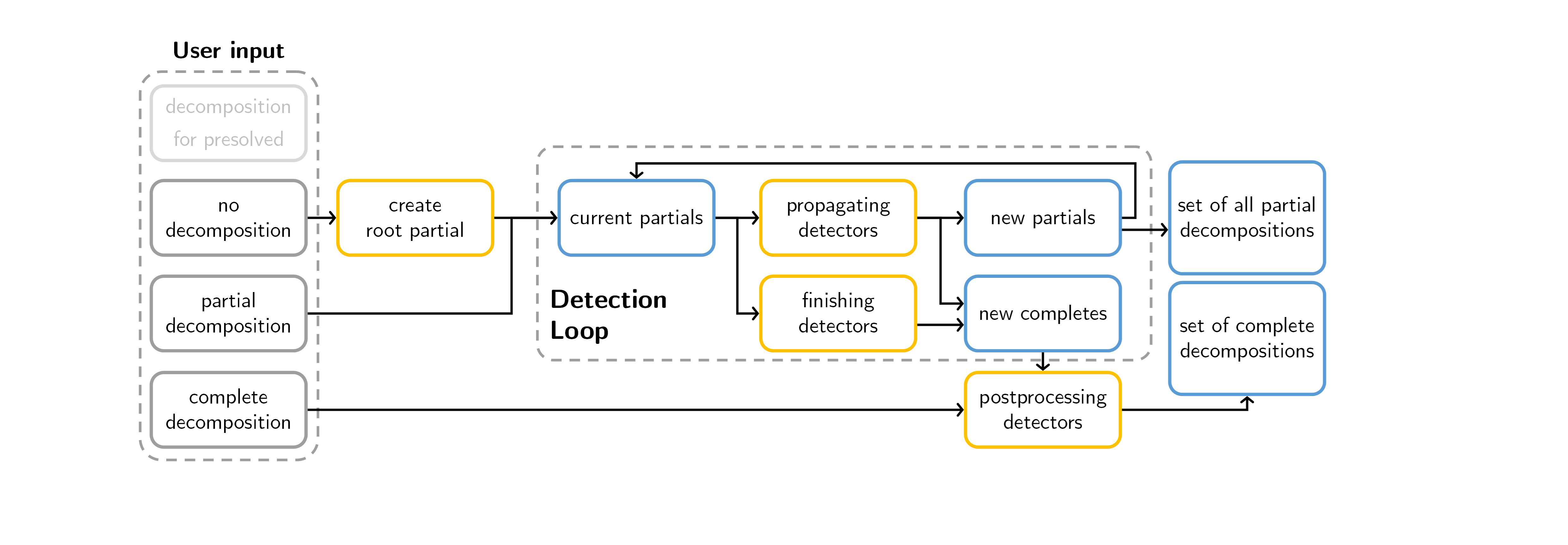
If your decomposition is complete, no detector can contribute anything anymore. Thus, GCG will not start The Detection Loop, but instead use the decomposition you gave and immediately start the solving.
If your decomposition is just partial, it is added to the (previously empty) pool of partial decompositions to use and GCG starts The Detection Loop. The procedure is clarified in the following section.

The Detection Loop

All detectors implemented in GCG assign variables/constraints to a block or the master. When the detection loop is started, a pool with partial decompositions is initialized, first with only one empty decomposition. Then, we start the loop. During this detection loop, we iterate over pairs of partial decompositions and detectors. This means that for each partial decomposition a detector yields (and the initial empty one), all other detectors will (potentially) work on this decomposition, completing it more and more with each iteration of the loop. It can happen that only one detector already completes a decomposition. After a number of iterations, the decomposition is complete and can be rated according to a score (see Detection Scores for a list of scores that can be set to be used). Then, the decomposition with the best score is used to proceed to the solving.

Before Presolving

After reading it in, the instance (the problem) you gave GCG is not presolved yet (see The GCG Presolving). To get decompositions that are not based on the presolved problem, you then have to perform a detect, since optimize will automatically execute a presolve first. Apart from that, you can also give an input, where there are three different cases that can happen:

• You don't give any decomposition.
• You have a rough idea of how your problem should be decomposed and give a partial decomposition.
• You know exactly how to decompose and give a complete decomposition.

Depending on those three cases, the detection runs differently. The exact process can be found in Figure 1.

Fig. 1: First stage of detection (problem is not yet presolved)

During/After Presolving

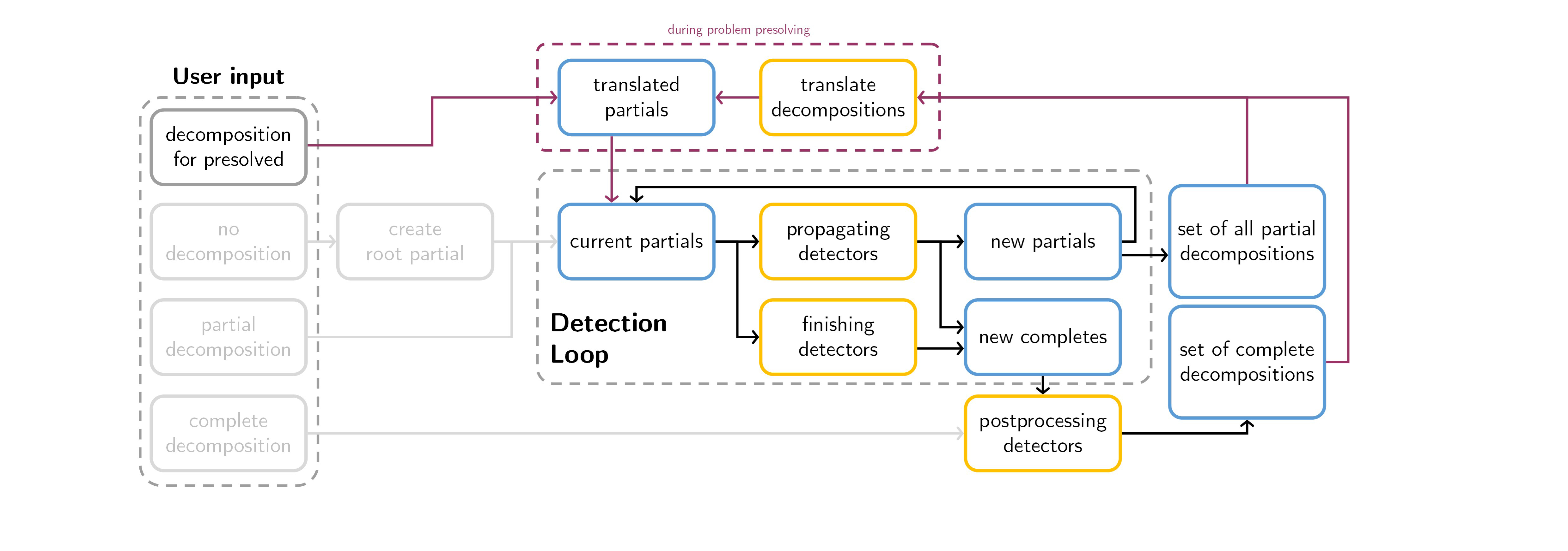
After the process shown in Figure 1 was executed, the problem you gave can also be presolved. If you just do an optimize, you will directly enter this case. In case you performed detect and optimize (as described above), you can now do a presolve in the interactive console. After presolving, some variables might have been aggregated or even removed and thus, the decompositions we found in the first run will be translated to match with the new, semantically equal, yet different problem. If you already knew how your problem would look like after presolving, you can also give a decomposition file for your problem - but presolved.
The detection process will then be executed as shown in Figure 2.

Fig. 2: Nonzero entries after decomposition

Standalone Capability of the Loop

A description of the standalone capabilities will follow soon.