
GCG
Branch-and-Price & Column Generation for Everyone
Branch-and-Price & Column Generation for Everyone
In this use case, we make GCG do the task it has been made for: solving structured mixed-integer programs. We will not go into any details concerning decomposition, reformulation or branch-and-price-and-cut, but only explain where one can find these steps in the output log and - just very superficially - what they mean.
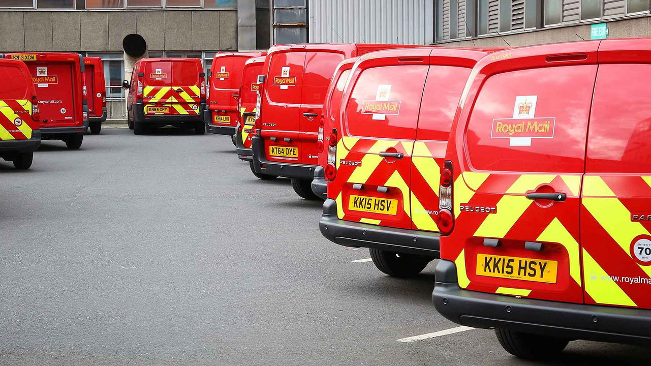
 This is Andrew. He lives near Edinburgh and has just founded his Start-up "Edin-OR" which specializes on optimizing planning and decision making processes within companies. Luckily, he has a friend over at Royal Mail, the local postal services company, who might help him with getting his first real job, scheduling the vehicles that deliver the mail. Since the management is doubtful of Andrew's capacilities, they ask him to begin with artificial data that is, however, very close to theirs. As a start, they suggest instances first used by Christofides et al. [2].
As always, Andrew starts with the exact problem definition.
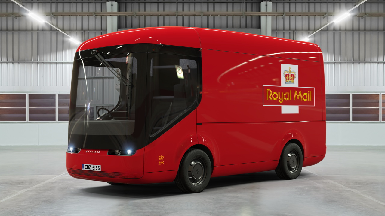
Sources: motoringresearch.com and electrek.co
The Royal Mail has a fleet consisting of about 50.000 vehicles and a subset of them operates in the Edinburgh region. Soon getting new, more efficient and environmentally-friendly electric vehicles, the local Royal Mail also wants to optimize the routes that they (and older vehicles) drive to deliver mail.
The goal is to deliver mail to all their customers using a given number of vehicles with limited capacity each. These will each drive their tour, starting from the depot and returning after their shift (after having delivered the mail to all recipients). Doing this, they don't have any time constraints, but instead just the capacity of their own vehicle. This is called the Capacitated Vehicle Routing Problem and has already been known for quite some time. A standard model is defined as following:
\begin{align} \min\quad & \sum_{(i,j) \in E} c_{ij}x_{ij}^{k}\\ s.t. \quad & \sum_{(i,j)\in \delta^{+} (i)} x_{ij}^{k}=\sum_{(j,i)\in \delta^{-} (i)} x_{ji}^{k}= \begin{cases} \begin{aligned} 1 &\qquad i=d,\\ z_{i}^{k} &\qquad i\neq d \end{aligned} \end{cases} \qquad && k \in \{1,\dots,K\}\\ & \sum_{k\in\{1,\dots,K\}} z_{i}^{k} = 1 && i\in V\\ & \sum_{(i,j)\in\delta^+(S)}x_{ij}\geq 1 \qquad && \emptyset \neq S \subsetneq V \\ & x_{ij}^{k} \in \{0,1\} && k\in\{1,\dots,K\},\ (i,j)\in E\\ & z_{i}^{k} \in \{0,1\} && k\in\{1,\dots,K\},\ i\in V\\ \end{align}
Andrew tries to choose an instance of medium difficulty to start with, even though they might become much bigger once he gets real data. The instance is called E021-06m. It features 21 customers to visit and 6 vehicles, each with a capacity of 4000. Note that the model by Christofides et al. is not exactly as the one above, since they refined it a bit further (see [2] for more information).
Andrew could also specify the problem himself using e.g. ZIMPL (see second use case).
With the problem at hand, Andrew starts searching for solvers of mixed integer programs. He quickly comes across the most common ones like Gurobi and SCIP. The latter has the advantage, that it is source-open and can be used without having to purchase a license, which is a big advantage because Andrew just wants do to a bit of testing and furthermore does not have that much capital yet (note that for commercial use of GCG and SCIP, the SCIP team has to be contacted first, since they require a different license). Thus, he tries to solve his instance with SCIP. After more than two hours he aborts the solving:
He thinks that he could do better, since Andrew knows that the problem at hand is a structured integer program. Thus, he starts searching for state-of-the-art methods for solving those. He encounters many proprietary approaches, where scientists had implemented their own customized solvers for their own vehicle routing and many other problems, but since Andrew has not yet gotten the hang of all this "decomposing", "pricing" or "cutting" and he also wants to reuse code as efficiently and often as possible, he starts looking for generic solvers that would do all of that automatically for him and finally finds "Generic Column Generation", which seems to be fitting. He is happy about the interface of GCG being just like those of all other commonly used solvers, but since the search for existing approaches had taken him so long, there is not much time left to solve the vehicle routing problem the management gave him, so he just goes ahead and installs GCG.
After the installation, Andrew fires up GCG with a simple
The output he is getting shows him the software versions and some copyright information. If he were to add more external code, which could improve solving speed, they would appear under "External Codes". As LP solver, he again can rely on the source-open solver "SoPlex", which, in contrast to "CPLEX" did not cost him anything. It is part of the whole SCIP Optimization Suite. Finally, he can see that the default settings are being used, which is fine, since he will not do any fine-tuning.
To continue, Andrew now wants to read in his problem. This can be done with a simple read and then the problem file. GCG will signalize that the problem was read successfully and already give some statistics: E021-06m only contains a few continuous variables and quite some integer variables and 2600 inequalities that are constraining the problem.
Finally, after looking at the Getting started Guide in GCG's documentation, he proceeds with optimizing his problem.
Having already worked with mixed integer programming solvers before, Andrew sees that there are many similarities to them. The optimal solution can be read at the bottom ("Primal Bound"), along with the time needed to solve it. If Andrew aborted before GCG was able to find an optimal solution, he would still be able to see the two bounds:
And would know that the objective function value of the optimal solution lies somewhere between 419 and 430. This result, which was obtained in just a few seconds, is already stronger than the two bounds that a non BP&C solver like SCIP calculated in over 2 hours (see above).
For many, this is not very relevant (they can just skip to the section Getting the Solution), but since Andrew wants to understand what is happening (at least someday), he takes a brief look at what was printed there. Before GCG starts with the "real" solving process (the Branch and Price and Cutting), there are a few steps that are executed and that distinguish GCG from other solvers.
More details and the corresponding theory and implementation can be found on the page The GCG Presolving.
During the presolving, trivially fulfilled or unsatisfied constraints are indentified as well as redundant variables and more. It can happen that a problem is already solved after presolving. The full log of a presolving process looks as following:
Andrew easily identifies that the presolving happens in rounds (1-7), where each round has different settings and different outcomes. Most importantly, in the line
he can see how variables and constraints were deleted and thus do not need to be respected anymore and the "bounds were tightened", meaning that these minor changes to his instance lead to a potentially faster solving of his problem.
More details and the corresponding theory and implementation can be found on the page The GCG Detection.
During the detection, one of GCG's main features, the solver will find different structures in your instance and will then "decompose" the problem such that it can be reformulated (see next section).
More details and the corresponding theory and implementation can be found on the page The GCG Pricing.
After decomposing the problem, GCG will apply a Dantzig-Wolfe (default) or Benders reformulation to the problem. With that formulation, the problem can in some cases be solved far more efficiently using Column Generation.
More details and the corresponding theory and implementation can be found on the page The GCG Pricing.
As a BP&C solver, GCG will apply Column Generation and apply cuts in every node of the branch-and-bound tree. Concerning the log, this is the part that Andrew already knows quite well. While most columns are not that important to him yet, there is one that is particularly, and that is the gap. It tells him how close GCG currently is to the optimal solution. It can also be read at the "dualbound" and "primalbound" columns.
Apart from the optimal objective function value, Andrew also wants to see which vehicle is routed where. To do this, he can simply (after having solved the problem) type display solution and will be able to see what values each variable has in the optimal solution.
Depending on the definition of the model, this can have different meanings, but here, the most intuitive applies: if x#1#3#1 is 1, then \(x^1_{31}=1\), i.e. vehicle \(1\) drives from customer \(3\) to customer \(1\). Since driving there is not free, this comes at a cost of about 8.06 units for the objective function value.
With this (not even that simple!) VRP instance, we were quite fortunate. SCIP does not seem to solve in reasonable time at all, and even commercial solvers such as gurobi are not faster than GCG. However, this is not always the case. It can happen that GCG performs significantly slower than other solvers not using Branch-and-Price. Thus, the main takeaway should be that you should always try column generation, since it can in many cases still be very beneficial to your solving performance. If you want to understand what the main factor of success of Branch-and-Price is, you should check out the page on Pricing Solvers.
 1.8.17